Tag: Distributions

  • Shapes of Distributions (Chapter 5)

    Probability distributions are fundamental concepts in statistics that describe how data is spread out or distributed. Understanding these distributions is crucial for students in fields ranging from social sciences to engineering. This essay will explore several key types of distributions and their characteristics.

    Normal Distribution

    The normal distribution, also known as the Gaussian distribution, is one of the most important probability distributions in statistics[1]. It is characterized by its distinctive bell-shaped curve and is symmetrical about the mean. The normal distribution has several key properties:

    1. The mean, median, and mode are all equal.
    2. Approximately 68% of the data falls within one standard deviation of the mean.
    3. About 95% of the data falls within two standard deviations of the mean.
    4. Roughly 99.7% of the data falls within three standard deviations of the mean.

    The normal distribution is widely used in natural and social sciences due to its ability to model many real-world phenomena.

    Skewness

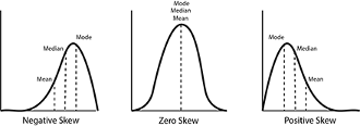
    Skewness is a measure of the asymmetry of a probability distribution. It indicates whether the data is skewed to the left or right of the mean[6]. There are three types of skewness:

    1. Positive skew: The tail of the distribution extends further to the right.
    2. Negative skew: The tail of the distribution extends further to the left.
    3. Zero skew: The distribution is symmetrical (like the normal distribution).

    Understanding skewness is important for students as it helps in interpreting data and choosing appropriate statistical methods.

    Kurtosis

    Kurtosis measures the “tailedness” of a probability distribution. It describes the shape of a distribution’s tails in relation to its overall shape. There are three main types of kurtosis:

    1. Mesokurtic: Normal level of kurtosis (e.g., normal distribution).
    2. Leptokurtic: Higher, sharper peak with heavier tails.
    3. Platykurtic: Lower, flatter peak with lighter tails.

    Kurtosis is particularly useful for students analyzing financial data or studying risk management[6].

    Bimodal Distribution

    A bimodal distribution is characterized by two distinct peaks or modes. This type of distribution can occur when:

    1. The data comes from two different populations.
    2. There are two distinct subgroups within a single population.

    Bimodal distributions are often encountered in fields such as biology, sociology, and marketing. Students should be aware that the presence of bimodality may indicate the need for further investigation into underlying factors causing the two peaks[8].

    Multimodal Distribution

    Multimodal distributions have more than two peaks or modes. These distributions can arise from:

    1. Data collected from multiple distinct populations.
    2. Complex systems with multiple interacting factors.

    Multimodal distributions are common in fields such as ecology, genetics, and social sciences. Students should recognize that multimodality often suggests the presence of multiple subgroups or processes within the data.

    In conclusion, understanding various probability distributions is essential for students across many disciplines. By grasping concepts such as normal distribution, skewness, kurtosis, and multi-modal distributions, students can better analyze and interpret data in their respective fields of study. As they progress in their academic and professional careers, this knowledge will prove invaluable in making informed decisions based on statistical analysis.

  • Distributions

    When working with datasets, it is important to understand the central tendency and dispersion of the data. These measures give us a general idea of how the data is distributed and what its typical values are. However, when the data is skewed or has outliers, it can be difficult to determine the central tendency and dispersion accurately. In this blog post, we’ll explore how to deal with skewed datasets and how to choose the appropriate measures of central tendency and dispersion.

    What is a Skewed Dataset?

    A skewed dataset is one in which the values are not evenly distributed. Instead, the data is skewed towards one end of the scale. There are two types of skewness: positive and negative. In a positive skewed dataset, the values are skewed to the right, while in a negative skewed dataset, the values are skewed to the left.

    Measures of Central Tendency

    Measures of central tendency are used to determine the typical value or center of a dataset. The three most commonly used measures of central tendency are the mean, median, and mode.

    1. Mean: The mean is the sum of all the values in the dataset divided by the number of values. It gives us an average value for the dataset.
    2. Median: The median is the middle value in a dataset. If the dataset has an odd number of values, the median is the value in the middle. If the dataset has an even number of values, the median is the average of the two middle values.
    3. Mode: The mode is the value that occurs most frequently in the dataset.

    In a skewed dataset, the mean is often skewed in the same direction as the data. This means that the mean may not accurately represent the typical value in a skewed dataset. In these cases, the median is often a better measure of central tendency. The median gives us the middle value in the dataset, which is not affected by outliers or skewness.

    Measures of Dispersion

    Measures of dispersion are used to determine how spread out the values in a dataset are. The two most commonly used measures of dispersion are the range and the standard deviation.

    1. Range: The range is the difference between the highest and lowest values in the dataset.
    2. Standard deviation: The standard deviation is a measure of how much the values in a dataset vary from the mean.

    In a skewed dataset, the range and standard deviation may be affected by outliers or skewness. In these cases, it is important to use other measures of dispersion, such as the interquartile range or trimmed mean, to get a more accurate representation of the dispersion in the data.

    When dealing with skewed datasets, it is important to choose the appropriate measures of central tendency and dispersion. The mean, median, and mode are measures of central tendency, while the range and standard deviation are measures of dispersion. In a skewed dataset, the mean may not accurately represent the typical value, and the range and standard deviation may be affected by outliers or skewness. In these cases, it is often better to use the median or other measures of dispersion to get a more accurate representation of the data.

  • Bi-Modal Distribution

    A bi-modal distribution is a statistical distribution that has two peaks in its frequency distribution curve, indicating that there are two distinct groups or subpopulations within the data set. These peaks can be roughly equal in size, or one peak may be larger than the other. In either case, the bi-modal distribution is a useful tool for identifying and analyzing patterns in data. 

    One example of a bi-modal distribution can be found in the distribution of heights among adult humans. The first peak in the distribution corresponds to the average height of adult women, which is around 5 feet 4 inches (162.6 cm). The second peak corresponds to the average height of adult men, which is around 5 feet 10 inches (177.8 cm). The two peaks in this distribution are clearly distinct, indicating that there are two distinct groups of people with different average heights. 

    To illustrate this bi-modal distribution, we can plot a frequency distribution histogram of heights of adult humans. The histogram would have two distinct peaks, one corresponding to the heights of women and the other corresponding to the heights of men. The histogram would also show that there is very little overlap between these two groups, indicating that they are largely distinct. 

    One of the main reasons why bi-modal distributions are important is that they can provide insights into the underlying structure of a data set. For example, in the case of the distribution of heights among adult humans, the bi-modal distribution indicates that there are two distinct groups with different average heights. This could be useful for a range of applications, from designing clothing to developing medical treatments. 

    Another example of a bi-modal distribution can be found in the distribution of income among households in the United States. The first peak in this distribution corresponds to households with low to moderate income, while the second peak corresponds to households with high income. This bi-modal distribution has been studied extensively by economists and policy makers, as it has important implications for issues such as income inequality and economic growth. 

    In conclusion, bi-modal distributions are a useful tool for identifying and analyzing patterns in data. They can provide insights into the underlying structure of a data set, and can be useful for a range of applications. The distribution of heights among adult humans and the distribution of income among households in the United States are two examples of bi-modal distributions that have important implications for a range of fields. A better understanding of bi-modal distributions can help us make better decisions and develop more effective solutions to complex problems.