how to set up a cross-sectional design in quantitative research in a media-related context:
Research Question: What is the relationship between social media use and body image satisfaction among teenage girls?
Define the research question: Determine the research question that the study will address. The research question should be clear, specific, and measurable.
Select the study population: Identify the population that the study will target. The population should be clearly defined and include specific demographic characteristics. For example, the population might be teenage girls aged 13-18 who use social media.
Choose the sampling strategy: Determine the sampling strategy that will be used to select the study participants. The sampling strategy should be appropriate for the study population and research question. For example, you might use a stratified random sampling strategy to select a representative sample of teenage girls from different schools in a specific geographic area.
Select the data collection methods: Choose the data collection methods that will be used to collect the data. The methods should be appropriate for the research question and study population. For example, you might use a self-administered questionnaire to collect data on social media use and body image satisfaction.
Develop the survey instrument: Develop the survey instrument based on the research question and data collection methods. The survey instrument should be valid and reliable, and include questions that are relevant to the research question. For example, you might develop a questionnaire that includes questions about the frequency and duration of social media use, as well as questions about body image satisfaction.
Collect the data: Administer the survey instrument to the study participants and collect the data. Ensure that the data is collected in a standardized manner to minimize measurement error.
Analyze the data: Analyze the data using appropriate statistical methods to answer the research question. For example, you might use correlation analysis to examine the relationship between social media use and body image satisfaction.
Interpret the results: Interpret the results and draw conclusions based on the findings. The conclusions should be based on the data and the limitations of the study. For example, you might conclude that there is a significant negative correlation between social media use and body image satisfaction among teenage girls, but that further research is needed to explore the causal mechanisms behind this relationship.
Research question: Does watching a 10-minute news clip on current events increase media literacy among undergraduate students?
Sample: Undergraduate students who are enrolled in media studies courses at a university
Before measurement: Administer a pre-test to assess students’ media literacy before watching the news clip. This could include questions about the credibility of sources, understanding of media bias, and ability to identify different types of media (e.g. news, opinion, entertainment).
Intervention: Ask students to watch a 10-minute news clip on current events, such as a segment from a national news program or a clip from a news website.
After measurement: Administer a post-test immediately after the news clip to assess any changes in media literacy. The same questions as the pre-test can be used to see if there were any significant differences in student understanding after watching the clip.
Analysis: Use statistical analysis, such as a paired t-test, to compare the pre- and post-test scores and determine if there was a statistically significant increase in media literacy after watching the news clip.For example, if the study finds that the average media literacy score increased significantly after watching the news clip, this would suggest that incorporating media clips into media studies courses could be an effective way to increase students’ understanding of media literacy
The independent t-test, also known as the two-sample t-test or unpaired t-test, is a fundamental statistical method used to assess whether the means of two unrelated groups are significantly different from one another. This inferential test is particularly valuable in various fields, including psychology, medicine, and social sciences, as it allows researchers to draw conclusions about population parameters based on sample data when the assumptions of normality and equal variances are met. Its development can be traced back to the early 20th century, primarily attributed to William Sealy Gosset, who introduced the concept of the t-distribution to handle small sample sizes, thereby addressing limitations in traditional hypothesis testing methods. The independent t-test plays a critical role in data analysis by providing a robust framework for hypothesis testing, facilitating data-driven decision-making across disciplines. Its applicability extends to real-world scenarios, such as comparing the effectiveness of different treatments or assessing educational outcomes among diverse student groups.
The test’s significance is underscored by its widespread usage and enduring relevance in both academic and practical applications, making it a staple tool for statisticians and researchers alike. However, the independent t-test is not without its controversies and limitations. Critics point to its reliance on key assumptions—namely, the independence of samples, normality of the underlying populations, and homogeneity of variances—as potential pitfalls that can compromise the validity of results if violated.
Moreover, the test’s sensitivity to outliers and the implications of sample size on generalizability further complicate its application, necessitating careful consideration and potential alternative methods when these assumptions are unmet. Despite these challenges, the independent t-test remains a cornerstone of statistical analysis, instrumental in hypothesis testing and facilitating insights across various research fields. As statistical practices evolve, ongoing discussions around its assumptions and potential alternatives continue to shape its application, reflecting the dynamic nature of data analysis methodologies in contemporary research.
Paper Digest is an AI-powered scholarly assistant designed to help researchers, students, and professionals navigate and analyze academic research more efficiently. Here are its key features and functions:
Main Functions
Research Paper Search and Summarization
Quickly find and summarize relevant academic papers
Provide detailed insights and key findings from scientific literature.
Assist in identifying the most recent and high-impact research in a specific field
Unique Features
No Hallucinations Guarantee: Ensures summaries are based on verifiable sources without fabricated information
Up-to-Date Data Integration: Continuously updates from hundreds of authoritative sources in real-time
Customizable search parameters allowing users to define research scope
NotebookLM is an experimental AI-powered research assistant developed by Google. Here are the key features and capabilities of NotebookLM:
NotebookLM allows users to consolidate and analyze information from multiple sources, acting as a virtual research assistant. Its main functions include:
Summarizing uploaded documents
Answering questions about the content
Generating insights and new ideas based on the source material
Creating study aids like quizzes, FAQs, and outlines
NotebookLM is particularly useful for:
Students and researchers synthesizing information from multiple sources
Content creators organizing ideas and generating scripts
Professionals preparing presentations or reports
Anyone looking to gain insights from complex or lengthy documents.
STORM (Synthesis of Topic Outlines through Retrieval and Multi-perspective Question Asking) is an innovative AI-powered research and writing tool developed by Stanford University. Launched in early 2024, STORM is designed to create comprehensive, Wikipedia-style articles on any given topic within minutes.
Key features of STORM include:
Automated content creation: STORM generates detailed, well-structured articles on a wide range of topics by leveraging large language models (LLMs) and simulating conversations between writers and topic experts.
Source referencing: Each piece of information is linked back to its original source, allowing for easy fact-checking and further exploration.
Multi-agent research: STORM utilizes a team of AI agents to conduct thorough research on the given topic, including research agents, question-asking agents, expert agents, and synthesis agents.
Open-source availability: As an open-source project, STORM is accessible to developers and researchers worldwide, fostering collaboration and continuous improvement.
Top-down writing approach: STORM employs a top-down approach, establishing the outline before writing content, which is crucial for effectively conveying information to readers.
STORM is particularly useful for academics, students, and content creators looking to craft well-researched articles quickly. It can serve as a valuable tool for finding research resources, conducting background research, and generating comprehensive overviews of various topics.
ChatGPT is an advanced artificial intelligence (AI) chatbot developed by OpenAI, designed to facilitate human-like conversations through natural language processing (NLP). Launched in November 2022, it utilizes a generative AI model called Generative Pre-trained Transformer (GPT), specifically the latest versions being GPT-4o and its mini variant. This technology enables ChatGPT to understand and generate text that closely resembles human conversation, allowing it to respond to inquiries, compose written content, and perform various tasks across different domains[1][2][5].
Applications of ChatGPT
The applications of ChatGPT are extensive:
Content Creation: Users leverage it to draft articles, blog posts, and marketing materials.
Educational Support: ChatGPT aids in answering questions and explaining complex topics in simpler terms.
Creative Writing: It generates poetry, scripts, and even music compositions.
Personal Assistance: Users can create lists for tasks or plan events with its help.
Limitations
Despite its capabilities, ChatGPT has limitations:
It may produce incorrect or misleading information.
Its knowledge base is capped at data available up until 2021 for some versions, limiting its awareness of recent events[4].
There are concerns regarding the potential for generating biased or harmful content.
Perplexity AI is an innovative conversational search engine designed to provide users with accurate and real-time answers to their queries. Launched in 2022 and based in San Francisco, California, it leverages advanced large language models (LLMs) to synthesize information from various sources on the internet, presenting it in a concise and user-friendly format.
use cases
Perplexity AI serves various purposes, such as:
Research and Information Gathering: It helps users conduct thorough research on diverse topics by allowing follow-up questions for deeper insights.
Content Creation: Users can utilize Perplexity for writing assistance, including summarizing articles or generating SEO content.
Project Management: The platform allows users to organize their queries into collections, making it suitable for managing research projects.
Fact-Checking: With its citation capabilities, Perplexity is useful for verifying facts and sources.
Napkin.AI is an innovative AI-driven tool designed to help users capture, organize, and visualize their ideas in a flexible and creative manner. Here are its key features and benefits:
Key Features
Idea Capturing and Organizing: Users can quickly jot down ideas as text or sketches, organizing them into clusters or timelines for better structure and understanding.
AI-Powered Insights: The platform utilizes AI to analyze notes and suggest connections, helping users discover relationships between ideas that may not be immediately apparent.
Visual Mapping: Napkin.AI allows the creation of mind maps and visual diagrams, making it easier to understand complex topics and relationships visually.
Text-to-Visual Conversion: Automatically transforms written content into engaging graphics, diagrams, and infographics, enhancing communication and storytelling.
Benefits
Flexible Workspace: The freeform nature of Napkin.AI allows for nonlinear thinking, making it ideal for creatives who prefer an open-ended approach to idea management.
Enhanced Creativity: AI-driven suggestions for linking ideas save time and inspire creativity by surfacing related concepts.
User-Friendly Interface: The clean design makes it easy for users of all skill levels to navigate the platform without a steep learning curve.
Napkin.AI combines these features to provide a powerful platform for individuals and teams looking to enhance their brainstorming sessions and project planning through visual thinking.
advanced AI-powered research tool designed to enhance the academic research experience. It offers a variety of features aimed at streamlining literature reviews and data analysis, making it a valuable resource for researchers, scholars, and students. Here are the key features and benefits:
Key Features
Comprehensive Literature Reviews
AnswerThis generates in-depth literature reviews by analyzing over 200 million research papers and reliable internet sources. This capability allows users to obtain relevant and up-to-date information tailored to their specific questions.
Source Summaries
The platform provides summaries of up to 20 sources for each literature review, including:
A comprehensive summary of each source.
Access to PDFs of the original papers when available.
Flexible Search Options
Users can perform searches with various filters such as:
Source type (research papers, internet sources, or personal library).
Time frame.
Field of study.
Minimum number of citations required.
Citation Management
The platform supports direct citations and allows users to export citations in multiple formats (e.g., APA, MLA, Chicago) for easy integration into their work).
Benefits
1. Time Efficiency
By automating the literature review process and summarizing complex papers, AnswerThis significantly saves time for researchers who would otherwise spend hours sifting through numerous sources.
2. Access to Credible Sources
The tool provides users with access to a wide range of credible academic sources, enhancing the quality and reliability of their research.
3. Enhanced Understanding
AnswerThis helps users understand intricate academic content through clear summaries and structured information, making it easier to grasp complex concepts.
offers several impressive features and benefits. Here are three key highlights:
Unlimited Transcriptions: TurboScribe allows users to transcribe an unlimited number of audio and video files, making it ideal for heavy usage without incurring additional costs12. This feature is particularly beneficial for professionals handling high-volume projects or individuals with frequent transcription needs.
High Accuracy and Speed: The tool boasts a remarkable 99.8% accuracy rate, powered by advanced AI technology23. It can convert files to text in seconds, significantly reducing the time spent on manual transcription and minimizing the need for extensive corrections34.
Multi-Language Support: TurboScribe supports transcription in over 98 languages and offers translation capabilities for more than 130 languages13. This extensive language support makes it an invaluable tool for global users, enabling efficient communication across language barriers and expanding its utility for international businesses, researchers, and content creators.
Gamma.ai
AI-powered content creation tool that offers several key functions and advantages:
AI-Driven Content Generation: Users can create presentations, documents, and websites quickly by entering text prompts or selecting templates[1][3]. The AI analyzes input and generates visually appealing, professional-quality content tailored to specific needs[3].
One-Click Polish and Restyle: Gamma.ai can refine rough drafts into polished presentations with a single click, handling formatting, styling, and aesthetics automatically[2].
Flexible Cards: The platform uses adaptable cards to condense complex topics while maintaining detail and context[2].
Real-Time Collaboration: Multiple users can work on a single project simultaneously, fostering team synergy and improving productivity[1].
Analytics Tools: Gamma.ai provides insights on audience engagement, helping users refine their presentations for better viewer resonance[1].
Unlimited Presentations: Users can create as many presentations as needed without restrictions, promoting creativity and productivity[1].
Integration Capabilities: The platform integrates with over 294 systems, improving workflow efficiency[1].
Data Visualization: Gamma.ai offers tools to help users effectively visualize data in their presentations[1].
Export Options: The platform allows for easy export of unlimited PDF and PPT files[5].
Sawtooth Software, 2021 Introduction to conjoint analysis Conjoint analysis is the premier approach for optimizing product features and pricing. It mimics the trade-offs people make in the real world when making choices. In conjoint analysis surveys you offer your respondents multiple alternatives with differing features… Lees meer: What is conjoint analysis?
Introduction In the field of media studies, understanding and reporting statistical significance is crucial for interpreting research findings accurately. Chapter 17 of “Introduction to Statistics in Psychology” by Howitt and Cramer provides valuable insights into the concise reporting of significance levels, a skill essential for… Lees meer: Reporting Significance levels (Chapter 17)
Chapter 16 of “Introduction to Statistics in Psychology” by Howitt and Cramer provides a foundational understanding of probability, which is crucial for statistical analysis in media research. For media students, grasping these concepts is essential for interpreting research findings and making informed decisions. This essay… Lees meer: Probability (Chapter 16)
The Chi-Square test, as introduced in Chapter 15 of “Introduction to Statistics in Psychology” by Howitt and Cramer, is a statistical method used to analyze frequency data. This guide will explore its core concepts and practical applications in media research, particularly for first-year media students.… Lees meer: Chi Square test (Chapter 15)
Unrelated T-Test: A Media Student’s Guide Chapter 14 of “Introduction to Statistics in Psychology” by Howitt and Cramer (2020) provides an insightful exploration of the unrelated t-test, a statistical tool that is particularly useful for media students analyzing research data. This discussion will delve into… Lees meer: Unrelated t-test (Chapter14)
Introduction The related t-test, also known as the paired or dependent samples t-test, is a statistical method extensively discussed in Chapter 13 of “Introduction to Statistics in Psychology” by Howitt and Cramer. This test is particularly relevant for media students as it provides a robust… Lees meer: Related t-test (Chapter13)
Understanding Correlation in Media Research: A Look at Chapter 8 Correlation analysis is a fundamental statistical tool in media research, allowing researchers to explore relationships between variables and draw meaningful insights. Chapter 8 of “Introduction to Statistics in Psychology” by Howitt and Cramer (2020) provides… Lees meer: Correlation (Chapter 8)
Exploring Relationships Between Multiple Variables: A Guide for Media Students In the dynamic world of media studies, understanding the relationships between multiple variables is crucial for analyzing audience behavior, content effectiveness, and media trends. This essay will explore various methods for visualizing and analyzing these… Lees meer: Relationships Between more than one variable (Chapter 7)
The standard deviation is a fundamental statistical concept that quantifies the spread of data points around the mean. It provides crucial insights into data variability and is essential for various statistical analyses. Calculation and Interpretation The standard deviation is calculated as the square root of… Lees meer: Standard Deviation (Chapter 6)
Here’s a guide on how to calculate the standard error in SPSS: Method 1: Using Descriptive Statistics Method 2: Using Frequencies Method 3: Using Compare Means Tips: Remember, the standard error is an estimate of how much the sample mean is likely to differ from… Lees meer: Guide SPSS How to: Calculate the Standard Error
Understanding Standard Error for Media Students Standard error is a crucial statistical concept that media students should grasp, especially when interpreting research findings or conducting their own studies. This essay will explain standard error and its relevance to media research, drawing from various sources and… Lees meer: Standard Error (Chapter 12)
Drawing strong conclusions in social research is a crucial skill for first-year students to master. Matthews and Ross (2010) emphasize that a robust conclusion goes beyond merely summarizing findings, instead addressing the critical “So What?” question by elucidating the broader implications of the research within… Lees meer: Drawing Conclusions (Chapter D10)
Research Methods in Social Research: A Comprehensive Guide to Data Collection Part C of “Research Methods: A Practical Guide for the Social Sciences” by Matthews and Ross focuses on the critical aspect of data collection in social research. This section provides a comprehensive overview of… Lees meer: Data Collection (Part C)
Research Methods in Social Research: Choosing the Right Approach The choice of research method in social research is a critical decision that shapes the entire study. Matthews and Ross (2010) emphasize the importance of aligning the research method with the research questions and objectives. They… Lees meer: Research Design (Chapter B3)
The choice of research method in social research is a critical decision that shapes the entire research process. Matthews and Ross (2010) emphasize the importance of aligning research methods with research questions and objectives. This alignment ensures that the chosen methods effectively address the research… Lees meer: Choosing Method(Chapter B4)
Here’s a step-by-step guide for 1st year students on how to calculate ANOVA in SPSS: Step 1: Prepare Your Data Step 2: Run the ANOVA Step 3: Additional Options Step 4: Post Hoc Tests Step 5: Run the Analysis Click “OK” in the main One-Way… Lees meer: Guide SPSS How to: Calculate ANOVA
Understanding Literature Reviews in Social Research(Theoretical Framework) A literature review is a crucial part of any social research project. It helps you build a strong foundation for your research by examining what others have already discovered about your topic. Let’s explore why it’s important and… Lees meer: Reviewing Literature (Chapter B2)
Chapter D6 Mathews and Ross Focus groups are a valuable qualitative research method that can provide rich insights into people’s thoughts, feelings, and experiences on a particular topic. As a university student, conducting focus groups can be an excellent way to gather data for research… Lees meer: Focus Groups (Chapter C5)
Chapter D4, Matthews and Ross Here is a guide on how to conduct a thematic analysis: What is Thematic Analysis? Thematic analysis is a qualitative research method used to identify, analyze, and report patterns or themes within data. It allows you to systematically examine a… Lees meer: Thematic Analysis (Chapter D4)
Probability distributions are fundamental concepts in statistics that describe how data is spread out or distributed. Understanding these distributions is crucial for students in fields ranging from social sciences to engineering. This essay will explore several key types of distributions and their characteristics. Normal Distribution… Lees meer: Shapes of Distributions (Chapter 5)
An Overview of Sampling Chapter 10 of the textbook, “Introduction to Statistics in Psychology,” focuses on the key concepts of samples and populations and their role in inferential statistics, which allows researchers to generalize findings from a smaller subset of data to the entire population… Lees meer: Podcast Sampling (Chapter 10)
Longitudinal research is a powerful research design that involves repeatedly collecting data from the same individuals or groups over a period of time, allowing researchers to observe how phenomena change and develop. Unlike cross-sectional studies, which capture a snapshot of a population at a single point in time, longitudinal research captures the dynamic nature of social life, providing a deeper understanding of cause-and-effect relationships, trends, and patterns.
Longitudinal studies can take on various forms, depending on the research question, timeframe, and resources available. Two common types are:
Prospective longitudinal studies: Researchers establish the study from the beginning and follow the participants forward in time. This approach allows researchers to plan data collection points and track changes as they unfold.
Retrospective longitudinal studies: Researchers utilize existing data from the past, such as medical records or historical documents, to construct a timeline and analyze trends over time. This approach can be valuable when studying events that have already occurred or when prospective data collection is not feasible.
Longitudinal research offers several advantages, including:
Tracking individual changes: By following the same individuals over time, researchers can observe how their attitudes, behaviors, or circumstances evolve, providing insights into individual growth and development.2
Identifying causal relationships: Longitudinal data can help establish the temporal order of events, strengthening the evidence for causal relationships.1 For example, a study that tracks individuals’ smoking habits and health outcomes over time can provide stronger evidence for the link between smoking and disease than a cross-sectional study.
Studying rare events or long-term processes: Longitudinal research is well-suited for investigating events that occur infrequently or phenomena that unfold over extended periods, such as the development of chronic diseases or the impact of social policies on communities.
However, longitudinal research also presents challenges:
Cost and time commitment: Longitudinal studies require significant resources and time investments, particularly for large-scale projects that span many years.
Data management: Collecting, storing, and analyzing data over time can be complex and require specialized expertise.
Attrition: Participants may drop out of the study over time due to various reasons, such as relocation, loss of interest, or death. Attrition can bias the results if those who drop out differ systematically from those who remain in the study.
Researchers utilize a variety of data collection methods in longitudinal studies, including surveys, interviews, observations, and document analysis. The choice of methods depends on the research question and the nature of the data being collected.
A key aspect of longitudinal research design is the selection of an appropriate sample. Researchers may use probability sampling techniques, such as stratified sampling, to ensure a representative sample of the population of interest. Alternatively, they may employ purposive sampling techniques to select individuals with specific characteristics or experiences relevant to the research question.
Millennium Cohort Study: This large-scale prospective study tracks the development of children born in the UK in the year 2000, collecting data on their health, education, and well-being at regular intervals.
Study on children’s experiences with smoking: This study employed both longitudinal and cross-sectional designs to examine how children’s exposure to smoking and their own smoking habits change over time.
Study on the experiences of individuals participating in an employment program: This qualitative study used longitudinal interviews to track participants’ progress and understand their experiences with the program over time.
Longitudinal research plays a crucial role in advancing our understanding of human behavior and social processes. By capturing change over time, these studies can provide valuable insights into complex phenomena and inform policy decisions, interventions, and theoretical development.
EXAMPLE SETUP
Research Question: Does exposure to social media impact the mental health of media students over time?
Hypothesis: Media students who spend more time on social media will experience a decline in mental health over time compared to those who spend less time on social media.
Methodology:
Participants: The study will recruit 100 media students, aged 18-25, who are currently enrolled in a media program at a university.
Data Collection: The study will collect data through online surveys administered at three time points: at the beginning of the study (Time 1), six months later (Time 2), and 12 months later (Time 3). The survey will consist of a series of questions about social media use (e.g., hours per day, types of social media used), as well as standardized measures of mental health (e.g., the Patient Health Questionnaire-9 for depression and the Generalized Anxiety Disorder-7 for anxiety).
Data Analysis: The study will use linear mixed-effects models to analyze the data, examining the effect of social media use on mental health outcomes over time while controlling for potential confounding variables (e.g., age, gender, prior mental health history).
Example Findings: After analyzing the data, the study finds that media students who spend more time on social media experience a significant decline in mental health over time compared to those who spend less time on social media. Specifically, students who spent more than 2 hours per day on social media at Time 1 experienced a 10% increase in depression symptoms and a 12% increase in anxiety symptoms at Time 3 compared to those who spent less than 1 hour per day on social media. These findings suggest that media students should be mindful of their social media use to protect their mental health
A cohort study is a specific type of longitudinal research design that focuses on a group of individuals who share a common characteristic, often their age or birth year, referred to as a cohort. Researchers track these individuals over time, collecting data at predetermined intervals to observe how their experiences, behaviors, and outcomes evolve. This approach enables researchers to investigate how various factors influence the cohort’s development and identify potential trends or patterns within the group12.
Cohort studies stand out for their ability to reveal changes within individuals’ lives, offering insights into cause-and-effect relationships that other research designs may miss. For example, a cohort study might track a group of students throughout their university experience to examine how alcohol consumption patterns change over time and relate those changes to academic performance, social interactions, or health outcomes3.
Researchers can design cohort studies on various scales and timeframes. Large-scale studies, such as the Millennium Cohort Study, often involve thousands of participants and continue for many years, requiring significant resources and a team of researchers2. Smaller cohort studies can focus on more specific events or shorter time periods. For instance, researchers could interview a group of people before, during, and after a significant life event, like a job loss or a natural disaster, to understand its impact on their well-being and coping mechanisms2.
There are two primary types of cohort studies:
Prospective cohort studies are established from the outset with the intention of tracking the cohort forward in time.
Retrospective cohort studies rely on existing data from the past, such as medical records or survey responses, to reconstruct the cohort’s history and analyze trends.
While cohort studies commonly employ quantitative data collection methods like surveys and statistical analysis, researchers can also incorporate qualitative methods, such as in-depth interviews, to gain a richer understanding of the cohort’s experiences. For example, in a study examining the effectiveness of a new employment program for individuals receiving disability benefits, researchers conducted initial in-depth interviews with participants and followed up with telephone interviews after three and six months to track their progress and gather detailed feedback4.
To ensure a representative and meaningful sample, researchers employ various sampling techniques in cohort studies. In large-scale studies, stratified sampling is often used to ensure adequate representation of different subgroups within the population25. For smaller studies or when specific characteristics are of interest, purposive sampling can be used to select individuals who meet certain criteria6.
Researchers must carefully consider the ethical implications of cohort studies, especially when working with vulnerable populations or sensitive topics. Ensuring informed consent, maintaining confidentiality, and minimizing potential harm to participants are paramount throughout the study7.
Cohort studies are a powerful tool for examining change over time and gaining insights into complex social phenomena. By meticulously tracking a cohort of individuals, researchers can uncover trends, identify potential causal relationships, and contribute valuable knowledge to various fields of study. However, researchers must carefully consider the challenges and ethical considerations associated with these studies to ensure their rigor and validity.
Research question: Start by defining a clear research question for each cohort, such as “What is the effect of social media use on the academic performance of first-year media students compared to third-year media students over a two-year period?”
Sampling: Decide on the population of interest for each cohort, such as first-year media students and third-year media students at a particular university, and then select a representative sample for each cohort. This can be done through a random sampling method or by selecting participants who meet specific criteria (e.g., enrolled in a particular media program and in their first or third year).
Data collection: Collect data from the participants in each cohort at the beginning of the study, and then at regular intervals over the two-year period (e.g., every six months). The data can be collected through surveys, interviews, or observation.
Variables: Identify the dependent and independent variables for each cohort. In this case, the independent variable would be social media use and the dependent variable would be academic performance (measured by GPA, test scores, or other academic indicators). For the second cohort, the time in the media program might also be a variable of interest.
Analysis: Analyze the data for each cohort separately using appropriate statistical methods to determine if there is a significant relationship between social media use and academic performance. This can include correlation analysis, regression analysis, or other statistical techniques.
Results and conclusions: Draw conclusions based on the analysis for each cohort and compare the results between the two cohorts. Determine if the results support or refute the research hypotheses for each cohort and make recommendations for future research or practical applications based on the findings.
Ethical considerations: Ensure that the study is conducted ethically for each cohort, with appropriate informed consent and confidentiality measures in place. Obtain necessary approvals from ethics committees or institutional review boards as required for each cohort
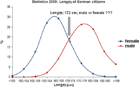
A bi-modal distribution is a statistical distribution that has two peaks in its frequency distribution curve, indicating that there are two distinct groups or subpopulations within the data set. These peaks can be roughly equal in size, or one peak may be larger than the other. In either case, the bi-modal distribution is a useful tool for identifying and analyzing patterns in data.
One example of a bi-modal distribution can be found in the distribution of heights among adult humans. The first peak in the distribution corresponds to the average height of adult women, which is around 5 feet 4 inches (162.6 cm). The second peak corresponds to the average height of adult men, which is around 5 feet 10 inches (177.8 cm). The two peaks in this distribution are clearly distinct, indicating that there are two distinct groups of people with different average heights.
To illustrate this bi-modal distribution, we can plot a frequency distribution histogram of heights of adult humans. The histogram would have two distinct peaks, one corresponding to the heights of women and the other corresponding to the heights of men. The histogram would also show that there is very little overlap between these two groups, indicating that they are largely distinct.
One of the main reasons why bi-modal distributions are important is that they can provide insights into the underlying structure of a data set. For example, in the case of the distribution of heights among adult humans, the bi-modal distribution indicates that there are two distinct groups with different average heights. This could be useful for a range of applications, from designing clothing to developing medical treatments.
Another example of a bi-modal distribution can be found in the distribution of income among households in the United States. The first peak in this distribution corresponds to households with low to moderate income, while the second peak corresponds to households with high income. This bi-modal distribution has been studied extensively by economists and policy makers, as it has important implications for issues such as income inequality and economic growth.
In conclusion, bi-modal distributions are a useful tool for identifying and analyzing patterns in data. They can provide insights into the underlying structure of a data set, and can be useful for a range of applications. The distribution of heights among adult humans and the distribution of income among households in the United States are two examples of bi-modal distributions that have important implications for a range of fields. A better understanding of bi-modal distributions can help us make better decisions and develop more effective solutions to complex problems.
Chapter 10 of the textbook, “Introduction to Statistics in Psychology,” focuses on the key concepts of samples and populations and their role in inferential statistics, which allows researchers to generalize findings from a smaller subset of data to the entire population of interest.
Population: The entire set of scores on a particular variable. It’s important to note that in statistics, the term “population” refers specifically to scores, not individuals or entities.
Sample: A smaller set of scores selected from the entire population. Samples are used in research due to the practical constraints of studying entire populations, which can be time-consuming and costly.
Random Samples and Their Characteristics
The chapter emphasizes the importance of random samples, where each score in the population has an equal chance of being selected. This systematic approach ensures that the sample is representative of the population, reducing bias and increasing the reliability of generalizations.
Various methods can be used to draw random samples, including using random number generators, tables, or even drawing slips of paper from a hat . The key is to ensure that every score has an equal opportunity to be included.
The chapter explores the characteristics of random samples, highlighting the tendency of sample means to approximate the population mean, especially with larger sample sizes. Tables 10.2 and 10.3 in the source illustrate this concept, demonstrating how the spread of sample means decreases and clusters closer to the population mean as the sample size increases.
Standard Error and Confidence Intervals
The chapter introduces standard error, a measure of the variability of sample means drawn from a population. Standard error is essentially the standard deviation of the sample means, reflecting the average deviation of sample means from the population mean.
Standard error is inversely proportional to the sample size. Larger samples tend to have smaller standard errors, indicating more precise estimates of the population mean.
The concept of confidence intervals is also explained. A confidence interval represents a range within which the true population parameter is likely to lie, based on the sample data. The most commonly used confidence level is 95%, meaning that there is a 95% probability that the true population parameter falls within the calculated interval .
Confidence intervals provide a way to quantify the uncertainty associated with inferring population characteristics from sample data. A wider confidence interval indicates greater uncertainty, while a narrower interval suggests a more precise estimate.
Key Points from Chapter 10
Understanding the distinction between samples and populations is crucial for applying inferential statistics.
Random samples are essential for drawing valid generalizations from research findings.
Standard error and confidence intervals provide measures of the variability and uncertainty associated with sample-based estimates of population parameters.
The chapter concludes by reminding readers that the concepts discussed serve as a foundation for understanding and applying inferential statistics in later chapters, paving the way for more complex statistical tests like t-tests .
In this blog post, we will discuss the basics of A/B testing and provide some examples of how media professionals can use it to improve their content.
What is A/B Testing?
A/B testing is a method of comparing two variations of a webpage, email, or advertisement to determine which performs better. The variations are randomly assigned to different groups of users, and their behavior is measured and compared to determine which variation produces better results. The goal of A/B testing is to identify which variations produce better results so that media professionals can make data-driven decisions for future content.
A/B Testing Examples
There are many different ways that media professionals can use A/B testing to optimize their content. Below are some examples of how A/B testing can be used in various media contexts.
Email Marketing
Email marketing is a popular way for media companies to engage with their audience and drive traffic to their website. A/B testing can be used to test different subject lines, email designs, and call-to-action buttons to determine which variations produce the best open and click-through rates.
For example, a media company could test two different subject lines for an email promoting a new article. One subject line could be straightforward and descriptive, while the other could be more creative and attention-grabbing. By sending these two variations to a sample of their audience, the media company can determine which subject line leads to more opens and clicks, and use that data to improve future email campaigns.
Website Design
A/B testing can also be used to optimize website design and user experience. By testing different variations of a webpage, media professionals can identify which elements lead to more engagement, clicks, and conversions.
If you’re a student, researcher, or professional working in the field of statistics, you’ve likely heard of Z-scores. But why use Z-scores in your data analysis? In this blog post, we’ll explain why Z-scores can be so beneficial to your data analysis and provide examples of how to use them in your quantitative research. By the end of this post, you’ll have a better understanding of why Z-scores are so important and how to use them in your research.
(Image Suggestion: A graph showing a data set represented by Z-scores, highlighting the transformation of the data points in relation to the mean and standard deviation.)
What are Z-Scores?
Are you interested in developing a better understanding of statistics and quantitative research? If so, you’ve come to the right place! Today, we will delve into the topic of Z-Scores and their significance in statistics.
Z-Scores are numerical scores that indicate how many standard deviations an observation is from the mean. In other words, a Z-Score of 0 represents a data point that is exactly equal to the mean. A Z-Score of 1 indicates data one standard deviation above the mean, while -1 represents data one standard deviation below the mean.
Using Z-Scores enables us to normalize our data and provide context for each value relative to all other values in our dataset. This facilitates the comparison of values from different distributions and helps to minimize bias when evaluating two groups or samples. Furthermore, it provides an overall measure of how distinct a given score is from the mean, which is particularly useful for identifying extreme outliers or determining relative standing within a group or sample.
Additionally, Z-Scores can also inform us about the probability of a specific value occurring within a dataset, taking its position relative to the mean into account. This additional feature enhances the usefulness of Z-Scores when interpreting quantitative research results. Each distribution has its own set of unique probabilities associated with specific scores, and understanding this information empowers us to make more informed decisions regarding our datasets and draw meaningful conclusions from them.
Understanding the Benefits of Using Z-Scores in Statistics
Are you searching for a method to compare two datasets or interpret statistical results? If so, using Z-scores could be the solution. Z-scores are a statistical tool employed to determine the distance of an individual measurement from the mean value in a given dataset. This facilitates data comparison across different sample sizes and distributions, as well as the identification of outliers and trends.
The use of Z-scores offers numerous advantages over alternative statistics like raw scores or percentages. For instance, as it is not affected by outliers or extremes, it can yield more accurate outcomes compared to raw scores. Moreover, it is non-directional, disregarding whether a score is above or below the mean, making result interpretation less complicated.
Utilizing Z-scores also permits the quantification of individual performance in relation to a larger group, offering valuable insights into data set variability. Additionally, it provides a simple way to identify subtle patterns and trends that might be overlooked using other quantitative analysis methods like linear regression or chi-square tests. Finally, when employed in hypothesis testing, Z-scores aid in calculating confidence intervals. This allows for more precise measurements of the level of confidence one can have in their conclusions based on the sample size and distribution type.
Overall, correct comprehension and application of Z-scores can deliver significant benefits in statistical research and analysis, empowering more accurate decision-making.
Examples of How to Use Z-Scores in Quantitative Research
In quantitative research, z-scores are a useful tool for analyzing data and making informed decisions. Z-scores allow you to compare variables from different distributions, quantify how much a value differs from the mean, and make statements about the significance of results for inference testing. They are also used to standardize data, which can be used for comparison purposes and detect outliers in data sets.
Z-scores can be especially helpful when looking at two or more sets of data by converting them to a common scale. Using z-scores allows you to compare and analyze data from different populations without having to adjust for differences in magnitude between the two datasets. Z-scores can also help you identify relationships between variables in your quantitative research study, as well as determine statistical significance between two or more sets of data.
In addition, z-scores can be used to standardize data within a population, which is important for making proper inferences about the data. Finally, z-scores can be used to calculate correlation coefficients that measure the degree of linear association between two variables. All these uses make z-scores an invaluable tool in quantitative research that should not be overlooked!
In Conclusion
Z-scores are powerful tools for data analysis and quantitative research, making them invaluable assets in any statistician’s arsenal. Their ability to standardize data across distributions, identify outliers, and measure correlation coefficients makes them must-haves for all statistical research. With a better understanding of Z-scores, you can make more informed decisions based on your data sets and draw meaningful conclusions from your quantitative research. So don’t wait – start utilizing the power of Z-scores to improve your results today!
Quantitative research is a type of research that deals with collecting, analyzing, and interpreting numerical data. It is a systematic and objective approach to study a research problem by using statistical and mathematical methods. Quantitative research aims to provide answers to research problems through empirical investigation and analysis of data.
Essentials of quantitative research include:
Research problem: The first step in conducting quantitative research is to identify a research problem. This involves understanding the problem that needs to be addressed and why it is important to study it. The research problem should be clearly defined, feasible to study, and relevant to the field of study.
Research objective: Once the research problem has been identified, the next step is to establish the research objectives. Research objectives are specific and measurable goals that the research aims to achieve. They outline what the research hopes to accomplish and what questions it aims to answer.
Research goal: The research goal is a more general and broader statement of what the research hopes to achieve. It outlines the overall purpose of the research and the expected outcome.
Research questions: The research questions are specific questions that the research aims to answer. They help to clarify the research objectives and provide a roadmap for conducting the research.
Hypothesis: A hypothesis is a statement that predicts the relationship between two or more variables. In quantitative research, hypotheses are used to test the validity of the research questions and objectives. The hypothesis provides a framework for collecting and analyzing data to determine if the research objectives have been met.
In conclusion, quantitative research is a systematic and objective approach to the study of research problems. The essentials of quantitative research include identifying a research problem, establishing research objectives, defining the research goal, formulating research questions, and developing a hypothesis. By following these steps, quantitative researchers can ensure that their research is well-structured and that they have a clear understanding of what they hope to achieve.