Tag: Quantitative

  • Standard Deviation (Chapter 6)

    The standard deviation is a fundamental statistical concept that quantifies the spread of data points around the mean. It provides crucial insights into data variability and is essential for various statistical analyses.

    Calculation and Interpretation

    The standard deviation is calculated as the square root of the variance, which represents the average squared deviation from the mean[1]. For a sample, the formula is:

    $$s = \sqrt{\frac{\sum_{i=1}^{n} (x_i – \bar{x})^2}{n – 1}}$$

    Where s is the sample standard deviation, x_i are individual values, $$\bar{x}$$ is the sample mean, and n is the sample size[1].

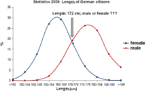
    Interpreting the standard deviation involves understanding its relationship to the mean and the overall dataset. A low standard deviation indicates that data points cluster closely around the mean, while a high standard deviation suggests a wider spread of values[1].

    Real-World Applications

    In finance, a high standard deviation of stock returns implies higher volatility and thus, a riskier investment. In research studies, it can reflect the spread of data, influencing the study’s reliability and validity[1].

    The Empirical Rule

    For normally distributed data, the empirical rule, or the 68-95-99.7 rule, provides a quick interpretation:

    • Approximately 68% of data falls within one standard deviation of the mean
    • About 95% falls within two standard deviations
    • Nearly 99.7% falls within three standard deviations[2]

    This rule helps in identifying outliers and understanding the distribution of data points.

    Standard Deviation vs. Other Measures

    While simpler measures like the mean absolute deviation (MAD) exist, the standard deviation is often preferred. It weighs unevenly spread samples more heavily, providing a more precise measure of variability[3]. For instance:

    ValuesMeanMean Absolute DeviationStandard Deviation
    Sample A: 66, 30, 40, 64501517.8
    Sample B: 51, 21, 79, 49501523.7

    The standard deviation differentiates the variability between these samples more effectively than the MAD[3].

    Z-Scores and the Standard Normal Distribution

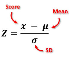
    Z-scores, derived from the standard deviation, indicate how many standard deviations a data point is from the mean. The formula is:

    $$z = \frac{x – \mu}{\sigma}$$

    Where x is the raw score, μ is the population mean, and σ is the population standard deviation[2].

    The standard normal distribution, with a mean of 0 and a standard deviation of 1, is crucial for probability calculations and statistical inference[2].

    Importance in Statistical Analysis

    The standard deviation is vital for:

    1. Describing data spread
    2. Comparing group variability
    3. Conducting statistical tests (e.g., t-tests, ANOVA)
    4. Performing power analysis for sample size determination[2]

    Understanding the standard deviation is essential for interpreting research findings, assessing data quality, and making informed decisions based on statistical analyses.

    Citations:
    [1] https://www.standarddeviationcalculator.io/blog/how-to-interpret-standard-deviation-results
    [2] https://statisticsbyjim.com/basics/standard-deviation/
    [3] https://www.scribbr.com/statistics/standard-deviation/
    [4] https://www.investopedia.com/terms/s/standarddeviation.asp
    [5] https://www.dummies.com/article/academics-the-arts/math/statistics/how-to-interpret-standard-deviation-in-a-statistical-data-set-169772/
    [6] https://www.bmj.com/about-bmj/resources-readers/publications/statistics-square-one/2-mean-and-standard-deviation
    [7] https://en.wikipedia.org/wiki/Standard_variance
    [8] https://www.businessinsider.com/personal-finance/investing/how-to-find-standard-deviation

  • Guide SPSS How to: Calculate the Standard Error

    Here’s a guide on how to calculate the standard error in SPSS:

    Method 1: Using Descriptive Statistics

    1. Open your dataset in SPSS.
    2. Click on “Analyze” in the top menu.
    3. Select “Descriptive Statistics” > “Descriptives”[1].
    4. Move the variable you want to analyze into the “Variables” box.
    5. Click on “Options”.
    6. Check the box next to “S.E. mean” (Standard Error of Mean)[1].
    7. Click “Continue” and then “OK”.
    8. The output will display the standard error along with other descriptive statistics.

    Method 2: Using Frequencies

    1. Go to “Analyze” > “Descriptive Statistics” > “Frequencies”[1][2].
    2. Move your variable of interest to the “Variable(s)” box.
    3. Click on “Statistics”.
    4. Check the box next to “Standard error of mean”[2].
    5. Click “Continue” and then “OK”.
    6. The output will show the standard error in the statistics table.

    Method 3: Using Compare Means

    1. Select “Analyze” > “Compare Means” > “Means”[1].
    2. Move your variable to the “Dependent List”.
    3. Click on “Options”.
    4. Select “Standard error of mean” from the statistics list.
    5. Click “Continue” and then “OK”.
    6. The output will display the standard error for your variable.

    Tips:

    • Ensure your data is properly coded and cleaned before analysis.
    • For accurate results, your sample size should be sufficiently large (typically n > 20)[4].
    • The standard error decreases as sample size increases, indicating more precise estimates[4].

    Remember, the standard error is an estimate of how much the sample mean is likely to differ from the true population mean[6]. It’s a useful measure for assessing the accuracy of your sample statistics.

    Citations:
    [1] https://www.youtube.com/watch?v=m1TlZ5hqmaQ
    [2] https://www.youtube.com/watch?v=VakRmc3c1O4
    [3] https://ezspss.com/how-to-calculate-mean-and-standard-deviation-in-spss/
    [4] https://www.scribbr.com/statistics/standard-error/
    [5] https://www.oecd-ilibrary.org/docserver/9789264056275-8-en.pdf?accname=guest&checksum=CB35D6CEEE892FF11AC9DE3C68F0E07F&expires=1730946573&id=id
    [6] https://www.ibm.com/docs/en/cognos-analytics/11.1.0?topic=terms-standard-error
    [7] https://s4be.cochrane.org/blog/2018/09/26/a-beginners-guide-to-standard-deviation-and-standard-error/
    [8] https://www.ibm.com/support/pages/can-i-compute-robust-standard-errors-spss

  • Choosing Method(Chapter B4)

    The choice of research method in social research is a critical decision that shapes the entire research process. Matthews and Ross (2010) emphasize the importance of aligning research methods with research questions and objectives. This alignment ensures that the chosen methods effectively address the research problem and yield meaningful results.

    Quantitative and qualitative research methods represent two distinct approaches to social inquiry. Quantitative research deals with numerical data and statistical analysis, aiming to test hypotheses and establish generalizable patterns[1]. It employs methods such as surveys, experiments, and statistical analysis of existing data[3]. Qualitative research, on the other hand, focuses on non-numerical data like words, images, and sounds to explore subjective experiences and attitudes[3]. It utilizes techniques such as interviews, focus groups, and observations to gain in-depth insights into social phenomena[1].

    The debate between quantitative and qualitative approaches has evolved into a recognition of their complementary nature. Mixed methods research, which combines both approaches, has gained prominence in social sciences. This approach allows researchers to leverage the strengths of both methodologies, providing a more comprehensive understanding of complex social issues[4]. For instance, a study might use surveys to gather quantitative data on trends, followed by in-depth interviews to explore the underlying reasons for these trends.

    When choosing research methods, several practical considerations come into play. Researchers must consider the type of data required, their skills and resources, and the specific research context[4]. The nature of the research question often guides the choice of method. For example, if the goal is to test a hypothesis or measure the prevalence of a phenomenon, quantitative methods may be more appropriate. Conversely, if the aim is to explore complex social processes or understand individual experiences, qualitative methods might be more suitable[2].

    It’s important to note that the choice of research method is not merely a technical decision but also reflects epistemological and ontological assumptions about the nature of social reality and how it can be studied[1]. Researchers should be aware of these philosophical underpinnings when selecting their methods.

    In conclusion, the choice of research method in social research is a crucial decision that requires careful consideration of research objectives, practical constraints, and philosophical assumptions. By thoughtfully selecting appropriate methods, researchers can ensure that their studies contribute meaningful insights to the field of social sciences.

    References:

    Matthews, B., & Ross, L. (2010). Research methods: A practical guide for the social sciences. Pearson Education.

    Scribbr. (n.d.). Qualitative vs. Quantitative Research | Differences, Examples & Methods.

    Simply Psychology. (2023). Qualitative vs Quantitative Research: What’s the Difference?

    National University. (2024). What Is Qualitative vs. Quantitative Study?

    Citations:
    [1] https://www.scribbr.com/methodology/qualitative-quantitative-research/
    [2] https://researcher.life/blog/article/qualitative-vs-quantitative-research/
    [3] https://www.simplypsychology.org/qualitative-quantitative.html
    [4] https://www.nu.edu/blog/qualitative-vs-quantitative-study/
    [5] https://pmc.ncbi.nlm.nih.gov/articles/PMC3327344/
    [6] https://www.thesoundhq.com/qualitative-vs-quantitative-research-better-together/
    [7] https://www.fullstory.com/blog/qualitative-vs-quantitative-data/
    [8] https://accelerate.uofuhealth.utah.edu/improvement/understanding-qualitative-and-quantitative-approac

  • Guide SPSS How to: Calculate ANOVA

    Here’s a step-by-step guide for 1st year students on how to calculate ANOVA in SPSS:

    Step 1: Prepare Your Data

    1. Open SPSS and enter your data into the Data View.
    2. Create two columns: one for your independent variable (factor) and one for your dependent variable (score)
    3. For the independent variable, use numbers to represent different groups (e.g., 1, 2, 3 for three different groups)

    Step 2: Run the ANOVA

    1. Click on “Analyze” in the top menu.
    2. Select “Compare Means” > “One-Way ANOVA”
    3. In the dialog box that appears:
    • Move your dependent variable (score) to the “Dependent List” box.
    • Move your independent variable (factor) to the “Factor” box

    Step 3: Additional Options

    1. Click on “Options” in the One-Way ANOVA dialog box.
    2. Select the following:
    • Descriptive statistics
    • Homogeneity of variance test
    • Means plot
    1. Click “Continue” to return to the main dialog box.

    Step 4: Post Hoc Tests

    1. Click on “Post Hoc” in the One-Way ANOVA dialog box
    2. Select “Tukey” for the post hoc test
    3. Ensure the significance level is set to 0.05 (unless your study requires a different level)
    4. Click “Continue” to return to the main dialog box.

    Step 5: Run the Analysis

    Click “OK” in the main One-Way ANOVA dialog box to run the analysis

    Step 6: Interpret the Results

    1. Check the “Test of Homogeneity of Variances” table. The significance value should be > 0.05 to meet this assumption
    2. Look at the ANOVA table:
    • If the significance value (p-value) is < 0.05, there are significant differences between groups
    1. If significant, examine the “Post Hoc Tests” table to see which specific groups differ
    2. Review the “Descriptives” table for means and standard deviations of each group

    Remember, ANOVA requires certain assumptions to be met, including normal distribution of the dependent variable and homogeneity of variances

    Always check these assumptions before interpreting your results.

  • Guide SPSS How to: Calculate the dependent t-test

    Here’s a guide for 1st year students on how to calculate the dependent t-test in SPSS:

    Step-by-Step Guide for Dependent t-test in SPSS

    1. Prepare Your Data

    • Ensure your data is in the correct format: two columns, one for each condition (e.g., before and after)
    • Each row should represent a single participant

    2. Open SPSS and Enter Data

    • Open SPSS and switch to the “Variable View”
    • Define your variables (e.g., “Before” and “After”)
    • Switch to “Data View” and enter your data

    3. Run the Test

    • Click on “Analyze” in the top menu
    • Select “Compare Means” > “Paired-Samples t Test”.
    • In the dialog box, move your two variables (e.g., Before and After) to the “Paired Variables” box
    • Click “OK” to run the test

    4. Interpret the Results

    • Look at the “Paired Samples Statistics” table for descriptive statistics
    • Check the “Paired Samples Test” table:
    • Find the t-value, degrees of freedom (df), and significance (p-value)
    • If p < 0.05, there’s a significant difference between the two conditions

    5. Report the Results

    • State whether there was a significant difference.
    • Report the t-value, degrees of freedom, and p-value.
    • Include means for both conditions.

    Tips:

    • Always check your data for accuracy before running the test.
    • Ensure your sample size is adequate for reliable results.
    • Consider the assumptions of the dependent t-test, such as normal distribution of differences between pairs.

    Remember, practice with sample datasets will help you become more comfortable with this process.

  • Guide SPSS How to: Calculate the independent t-test

    Step-by-Step Guide

    1. Open your SPSS data file.
    2. Click on “Analyze” in the top menu, then select “Compare Means” > “Independent-Samples T Test”
    3. In the dialog box that appears:
    • Move your dependent variable (continuous) into the “Test Variable(s)” box.
    • Move your independent variable (categorical with two groups) into the “Grouping Variable” box
    1. Click on the “Define Groups” button next to the Grouping Variable box
    2. In the new window, enter the values that represent your two groups (e.g., 0 for “No” and 1 for “Yes”)[1].
    3. Click “Continue” and then “OK” to run the test

    Interpreting the Results

    1. Check Levene’s Test for Equality of Variances:
    • If p > 0.05, use the “Equal variances assumed” row.
    • If p ≤ 0.05, use the “Equal variances not assumed” row
    1. Look at the “Sig. (2-tailed)” column:
    • If p ≤ 0.05, there is a significant difference between the groups.
    • If p > 0.05, there is no significant difference
    1. If significant, compare the means in the “Group Statistics” table to see which group has the higher score

    Tips

    • Ensure your data meets the assumptions for an independent t-test, including normal distribution and independence of observations
    • Consider calculating effect size, as SPSS doesn’t provide this automatically

  • Guide SPSS How to: Calculate Chi Square

    1. Open your data file in SPSS.
    2. Click on “Analyze” in the top menu, then select “Descriptive Statistics” > “Crosstabs”
    3. In the Crosstabs dialog box:
    • Move one categorical variable into the “Row(s)” box.
    • Move the other categorical variable into the “Column(s)” box.
    1. Click on the “Statistics” button and check the box for “Chi-square”
    2. Click on the “Cells” button and ensure “Observed” is checked under “Counts”
    3. Click “Continue” and then “OK” to run the analysis.

    Interpreting the Results

    1. Look for the “Chi-Square Tests” table in the output
    2. Find the “Pearson Chi-Square” row and check the significance value (p-value) in the “Asymptotic Significance (2-sided)” column
    3. If the p-value is less than your chosen significance level (typically 0.05), you can reject the null hypothesis and conclude there is a significant association between the variables

    Main Weakness of Chi-square Test

    The main weakness of the Chi-square test is its sensitivity to sample size[3]. Specifically:

    1. Assumption violation: The test assumes that the expected frequency in each cell should be 5 or more in at least 80% of the cells, and no cell should have an expected frequency of less than 1
    2. Sample size issues:
    • With small sample sizes, the test may not be valid as it’s more likely to violate the above assumption.
    • With very large sample sizes, even small, practically insignificant differences can appear statistically significant.

    To address this weakness, always check the “Expected Count” in your output to ensure the assumption is met. If not, consider combining categories or using alternative tests for small samples, such as Fisher’s Exact Test for 2×2 tables

  • Guide SPSS How to: Correlation

    Calculating Correlation in SPSS

    Step 1: Prepare Your Data

    • Enter your data into SPSS, with each variable in a separate column.
    • Ensure your variables are measured on an interval or ratio scale for Pearson’s r, or ordinal scale for Spearman’s rho

    Step 2: Access the Correlation Analysis Tool

    1. Click on “Analyze” in the top menu.
    2. Select “Correlate” from the dropdown menu.
    3. Choose “Bivariate” from the submenu

    Step 3: Select Variables

    • In the new window, move your variables of interest into the “Variables” box.
    • You can select multiple variables to create a correlation matrix

    Step 4: Choose Correlation Coefficient

    • For Pearson’s r: Ensure “Pearson” is checked (it’s usually the default).
    • For Spearman’s rho: Check the “Spearman” box

    Step 5: Additional Options

    • Under “Test of Significance,” select “Two-tailed” unless you have a specific directional hypothesis.
    • Check “Flag significant correlations” to highlight significant results

    Step 6: Run the Analysis

    • Click “OK” to generate the correlation output

    Interpreting the Results

    Correlation Coefficient

    • The value ranges from -1 to +1.
    • Positive values indicate a positive relationship, negative values indicate an inverse relationship[1].
    • Strength of correlation:
    • 0.00 to 0.29: Weak
    • 0.30 to 0.49: Moderate
    • 0.50 to 1.00: Strong

    Statistical Significance

    • Look for p-values less than 0.05 (or your chosen significance level) to determine if the correlation is statistically significant.

    Sample Size

    • The output will also show the sample size (n) for each correlation.

    Remember, correlation does not imply causation. Always interpret your results in the context of your research question and theoretical framework.

    To interpret the results of a Pearson correlation in SPSS, focus on these key elements:

    1. Correlation Coefficient (r): This value ranges from -1 to +1 and indicates the strength and direction of the relationship between variables
    • Positive values indicate a positive relationship, negative values indicate an inverse relationship.
    • Strength interpretation:
      • 0.00 to 0.29: Weak correlation
      • 0.30 to 0.49: Moderate correlation
      • 0.50 to 1.00: Strong correlation
    1. Statistical Significance: Look at the “Sig. (2-tailed)” value
    • If this value is less than your chosen significance level (typically 0.05), the correlation is statistically significant.
    • Significant correlations are often flagged with asterisks in the output.
    1. Sample Size (n): This indicates the number of cases used in the analysis

    Example Interpretation

    Let’s say you have a correlation coefficient of 0.228 with a significance value of 0.060:

    1. The correlation coefficient (0.228) indicates a weak positive relationship between the variables.
    2. The significance value (0.060) is greater than 0.05, meaning the correlation is not statistically significant
    3. This suggests that while a small positive correlation was observed in the sample, there’s not enough evidence to conclude that this relationship exists in the population
    4. Remember, correlation does not imply causation. Always interpret results in the context of your research question and theoretical framework.

  • Anova and Manova

    Exploring ANOVA and MANOVA Techniques in Marketing and Media Studies

    Analysis of Variance (ANOVA) and Multivariate Analysis of Variance (MANOVA) are powerful statistical tools that can provide valuable insights for marketing and media studies. Let’s explore these techniques with relevant examples for college students in these fields.

    Repeated Measures ANOVA

    Repeated Measures ANOVA is used when the same participants are measured multiple times under different conditions. This technique is particularly useful in marketing and media studies for assessing changes in consumer behavior or media consumption over time or across different scenarios.

    Example for Marketing Students:
    Imagine a study evaluating the effectiveness of different advertising formats (TV, social media, print) on brand recall. Participants are exposed to all three formats over time, and their brand recall is measured after each exposure. The repeated measures ANOVA would help determine if there are significant differences in brand recall across these advertising formats.

    The general formula for repeated measures ANOVA is:

    $$F = \frac{MS_{between}}{MS_{within}}$$

    Where:

    • $$MS_{between}$$ is the mean square between treatments
    • $$MS_{within}$$ is the mean square within treatments

    MANOVA

    MANOVA extends ANOVA by allowing the analysis of multiple dependent variables simultaneously. This is particularly valuable in marketing and media studies, where researchers often want to examine the impact of independent variables on multiple outcome measures.

    Example for Media Studies:
    Consider a study investigating the effects of different types of news coverage (positive, neutral, negative) on viewers’ emotional responses and information retention. The dependent variables could be:

    1. Emotional response (measured on a scale)
    2. Information retention (measured by a quiz score)
    3. Likelihood to share the news (measured on a scale)

    MANOVA would allow researchers to analyze how the type of news coverage affects all these outcomes simultaneously.

    The most commonly used test statistic in MANOVA is Pillai’s trace, which can be represented as:

    $$V = \sum_{i=1}^s \frac{\lambda_i}{1 + \lambda_i}$$

    Where:

    • $$V$$ is Pillai’s trace
    • $$\lambda_i$$ are the eigenvalues of the matrix product of the between-group sum of squares and cross-products matrix and the inverse of the within-group sum of squares and cross-products matrix
    • $$s$$ is the number of eigenvalues

    Discriminant Function Analysis and MANOVA

    After conducting a MANOVA, discriminant function analysis can help identify which aspects of the dependent variables contribute most to group differences.

    Marketing Example:
    In a study of consumer preferences for different product attributes (price, quality, brand reputation), discriminant function analysis could reveal which combination of these attributes best distinguishes between different consumer segments.

    Reporting MANOVA Results

    When reporting MANOVA results, include:

    1. The specific multivariate test used (e.g., Pillai’s trace)
    2. F-statistic, degrees of freedom, and p-value
    3. Interpretation in the context of your research question

    Example: “A one-way MANOVA revealed a significant multivariate main effect for news coverage type, Pillai’s trace = 0.38, F(6, 194) = 7.62, p < .001, partial η2 = .19.”

    Conclusion

    ANOVA and MANOVA techniques offer powerful tools for marketing and media studies students to analyze complex datasets involving multiple variables. By understanding these methods, students can design more sophisticated studies and draw more nuanced conclusions about consumer behavior, media effects, and market trends[1][2][3][4][5].

    Citations:
    [1] https://fastercapital.com/content/MANOVA-and-MANCOVA–Marketing-Mastery–Unleashing-the-Potential-of-MANOVA-and-MANCOVA.html
    [2] https://fastercapital.com/content/MANOVA-and-MANCOVA–MANOVA-and-MANCOVA–A-Strategic-Approach-for-Marketing-Research.html
    [3] https://www.proquest.com/docview/1815499254
    [4] https://business.adobe.com/blog/basics/multivariate-analysis-examples
    [5] https://www.worldsupporter.org/en/summary/when-and-how-use-manova-and-mancova-chapter-7-exclusive-86003
    [6] https://www.linkedin.com/advice/0/how-can-you-use-manova-analyze-impact-advertising-35cbf
    [7] https://methods.sagepub.com/video/an-introduction-to-manova-and-mancova-for-marketing-research
    [8] https://www.researchgate.net/publication/2507074_MANOVAMAP_Graphical_Representation_of_MANOVA_in_Marketing_Research

  • Data Analysis (Section D)

    Ever wondered how researchers make sense of all the information they collect? Section D of Matthews and Ross’ book is your treasure map to the hidden gems in data analysis. Let’s embark on this adventure together!

    Why Analyze Data?

    Imagine you’re a detective solving a mystery. You’ve gathered all the clues (that’s your data), but now what? Data analysis is your magnifying glass, helping you piece together the puzzle and answer your burning research questions.

    Pro Tip: Plan Your Analysis Strategy Early!

    Before you start collecting data, decide how you’ll analyze it. It’s like choosing your weapon before entering a video game battle – your data collection method will determine which analysis techniques you can use.

    Types of Data: A Trilogy

    1. Structured Data: The neat freak of the data world. Think multiple-choice questionnaires – easy to categorize and analyze.
    2. Unstructured Data: The free spirit. This could be interviews or open-ended responses – more challenging but often rich in insights.
    3. Semi-structured Data: The best of both worlds. A mix of structured and unstructured elements.

    Crunching Numbers: Statistical Analysis

    For all you number lovers out there, statistical analysis is your playground. Learn to summarize data, spot patterns, and explore relationships between different factors. It’s like being a data detective!

    Thematic Analysis: Finding the Hidden Threads

    This is where you become a storyteller, weaving together themes and patterns from qualitative data. Pro tip: Keep a research diary to track your “Eureka!” moments.

    Beyond the Basics: Other Cool Techniques

    • Narrative Analysis: Decoding the stories people tell
    • Discourse Analysis: Understanding how language shapes reality
    • Content Analysis: Counting words to uncover meaning
    • Grounded Theory: Building theories from the ground up

    Tech to the Rescue: Computers in Data Analysis

    Say goodbye to manual number crunching! Learn about software like SPSS and NVivo that can make your analysis life much easier.

    The Grand Finale: Drawing Conclusions

    This is where you answer the ultimate question: “So what?” What does all this analysis mean, and why should anyone care?

    Remember, data analysis isn’t just about crunching numbers or coding text. It’s about uncovering insights that can change the world. So, are you ready to become a data analysis superhero? Let’s get started!