Laddering Theory, Method, Analysis, and Interpretation by Thomas J. Reynolds and Jonathan Gutman is a foundational framework in qualitative research, particularly within consumer behavior studies. Below is an overview of the key aspects of this theory and methodology:
Overview of Laddering Theory
Laddering is a qualitative research technique designed to uncover the deeper motivations, values, and decision-making processes underlying consumer behavior. It is rooted in the Means-End Chain Theory, which posits that consumers make choices based on a hierarchy of perceptions involving three levels:
Attributes (A): The tangible or intangible features of a product or service.
Consequences (C): The outcomes or benefits derived from those attributes.
Values (V): The personal values or life goals that these consequences serve[1][4].
The laddering process seeks to identify the connections between these levels (A → C → V) to understand how products or services align with consumers’ personal values.
Methodology
The laddering technique involves in-depth, one-on-one interviews using a structured probing approach. The primary question format revolves around asking “Why is that important to you?” repeatedly to move from surface-level attributes to deeper values. This process creates a “ladder” of associations for each respondent[1][2][4].
Steps in Laddering:
Eliciting Attributes: Start by identifying the key features that differentiate a product or service.
Identifying Consequences: Probe to understand the benefits or outcomes associated with these attributes.
Uncovering Values: Further probe to reveal the personal values tied to these consequences.
Data Analysis
Responses are analyzed using content analysis techniques to summarize key elements at each level of abstraction (A, C, V).
Results are visualized through a Hierarchical Value Map (HVM), which graphically represents the dominant linkages across attributes, consequences, and values[1][4].
Applications
The laddering method has been widely applied in marketing and consumer research to:
Develop effective branding strategies.
Understand consumer decision-making processes.
Identify opportunities for product innovation.
It provides insights into how consumers perceive products in relation to their self-concept and life goals, enabling businesses to align their offerings with consumer values[1][2][6].
Contributions by Reynolds and Gutman
Thomas J. Reynolds: A professor and researcher specializing in strategic positioning and communication options.
Jonathan Gutman: A marketing professor focused on developing and applying Means-End Chain methodology.
Their work has been instrumental in advancing both academic and practical applications of laddering as a robust tool for understanding consumer behavior[4].
Conjoint analysis is the premier approach for optimizing product features and pricing. It mimics the trade-offs people make in the real world when making choices. In conjoint analysis surveys you offer your respondents multiple alternatives with differing features and ask which they would choose.
With the resulting data, you can predict how people would react to any number of product designs and prices. Because of this, conjoint analysis is used as the advanced tool for testing multiple features at one time when A/B testing just doesn’t cut it.
Conjoint analysis is commonly used for:
Designing and pricing products / Healthcare and medical decisions / Branding, package design, and product claims / Environmental impact studies / Needs-based market segmentation
How does conjoint analysis work?
Step 1: Break products into attributes and levels
In the picture below, a conjoint analysis example, the attributes of a car are broken down into brand, engine, type, and price. Each of those attributes has different levels.
Rather than directly ask survey respondents what they prefer in a product, or what attributes they find most important, conjoint analysis employs the more realistic context of asking respondents to evaluate potential product profiles (see below).
Step 2: Show product profiles to respondents
Each profile includes multiple conjoined product features (hence, conjoint analysis), such as price, size, and color, each with multiple levels, such as small, medium, and large.
In a conjoint exercise, respondents usually complete between 8 to 20 conjoint questions. The questions are designed carefully, using experimental design principles of independence and balance of the features.
Step 3: Quantify your market’s preferences and create a model
By independently varying the features that are shown to the respondents and observing the responses to the product profiles, the analyst can statistically deduce what product features are most desired and which attributes have the most impact on choice (see below).
Screenshot
In contrast to simpler survey research methods that directly ask respondents what they prefer or the importance of each attribute, these preferences are derived from these relatively realistic trade-off situations.
The result is usually a full set of preference scores (often called part-worth utilities) for each attribute level included in the study. The many reporting options allow you to see which segments (or even individual respondents) are most likely to prefer your product (see example table).
Why use conjoint analysis?
When people face challenging trade-offs, we learn what’s truly important to them. Conjoint analysis doesn’t allow people to say that everything is important, which can happen in typical rating scale questions, but rather forces them to choose between competing realistic options. By systematically varying product features and prices in a conjoint survey and recording how people choose, you gain information that far exceeds standard concept testing.
If you want to predict how people will react to new product formulations or prices, you cannot rely solely on existing sales data, social media content, qualitative inquiries, or expert opinion.
What-if market simulators are a key reason decision-makers embrace and continue to request conjoint analysis studies. With the model built from choices in the conjoint analysis, market simulators allow managers to test feature/pricing combinations in a simulated shopping/choice environment to predict how the market would react.
What are the outputs of Conjoint Analysis?
The preference scores that result from a conjoint analysis are called utilities. The higher the utility, the higher the preference. Although you could report utilities to others, they are not as easy to interpret as the results of market simulations that are market choices summing to 100%.
Attribute importances are another traditional output from conjoint analysis. Importances sum to 100% across attributes and reflect the relative impact each attribute has on product choices. Attribute importances can be misleading in certain cases, however, because the range of levels you choose to include in the experiment have a strong effect on the resulting importance score.
The key deliverable is the what-if market simulator. This is a decision tool that lets you test thousands of different product formulations and pricing against competition and see what buyers will likely choose. Make a change to your product or price and run the simulation again to see the effect on market choices. You can use our market simulator application or our software can export your market simulator as an Excel sheet.
How are outputs used?
Companies use conjoint analysis tools to test improvements to their product, help them set profit-maximizing prices, and to guide their development of multiple product offerings to appeal to different market segments. Because graphics may be used as attribute levels, CPG firms use conjoint analysis to help design product packaging, colors, and claims. Economists use conjoint analysis for a variety of consumer decisions involving green energy choice, healthcare, or transportation. The possibilities are endless.
The Basics of Interpreting Conjoint Utilities
Users of conjoint analysis are sometimes confused about how to interpret utilities. Difficulty most often arises in trying to compare the utility value for one level of an attribute with a utility value for one level of another attribute. It is never correct to compare a single value for one attribute with a single value from another. Instead, one must compare differences in values. The following example illustrates this point:
Brand A 40 Red 20 $ 50 90 Brand B 60 Blue 10 $ 75 40 Brand C 20 Pink 0 $ 100 0
It is not correct to say that Brand C has the same desirability as the color Red. However, it is correct to conclude that the difference in value between brands B and A (60-40 = 20) is the same as the difference in values between Red and Pink (20-0 = 20). This respondent should be indifferent between Brand A in a Red color (40+20=60) and Brand B in a Pink color (60+ 0 = 60).
< see next page >
Sometimes we want to characterize the relative importance of each attribute. We do this by considering how much difference each attribute could make in the total utility of a product. That difference is the range in the attribute’s utility values. We percentage those ranges, obtaining a set of attribute importance values that add to 100, as follows:
Screenshot
For this respondent, the importance of Brand is 26.7%, the importance of Color is 13.3%, and the importance of Price is 60%. Importances depend on the particular attribute levels chosen for the study. For example, with a narrower range of prices, Price would have been less important.
When summarizing attribute importances for groups, it is best to compute importances for respondents individually and then average them, rather than computing importances using average utilities. For example, suppose we were studying two brands, Coke and Pepsi. If half of the respondents preferred each brand, the average utilities for Coke and Pepsi would be tied, and the importance of Brand would appear to be zero!
Source:
Sawtooth Software (2021), What is conjoint analysis [online], accessed 11-10-2021, available at: https://sawtoothsoftware.com/conjoint-analysis
To measure loss aversion among consumers in marketing, you can use the following approaches:
1. **Behavioral Experiments**:
Design experiments where participants choose between options framed as potential losses or gains. For example, test whether consumers are more likely to act when told they could “lose $10” versus “gain $10” for the same decision[2][6].
2. **A/B Testing in Campaigns**:
Run A/B tests by framing marketing messages differently. For instance, compare responses to “Limited-time offer: Don’t miss out!” versus “Exclusive deal: Act now to save!” Measure the impact on conversion rates, click-through rates, and customer actions[5][6].
3. **Surveys and Questionnaires**:
Use structured surveys to assess consumer preferences under loss- and gain-framed scenarios. Include questions about emotional responses to hypothetical losses versus gains[7].
4. **Endowment Effect Studies**:
Offer trial periods or temporary ownership of products and observe whether consumers are reluctant to give them up, indicating loss aversion[3].
5. **Field Studies**:
Analyze real-world data, such as changes in purchasing behavior during limited-time offers or stock scarcity alerts. Metrics like urgency-driven purchases can reflect loss aversion tendencies[1][5].
By combining these methods with analytics tools to track consumer behavior, you can quantify and leverage loss aversion effectively in marketing strategies.
Sources
[1] The Power Of Loss Aversion In Marketing: A Comprehensive Guide https://www.linkedin.com/pulse/power-loss-aversion-marketing-comprehensive-guide-james-taylor- [2] Using the Theory of Loss Aversion in Marketing To Gain … – Brax.io https://www.brax.io/blog/using-loss-aversion-in-marketing-to-gain-more-customers [3] What is loss aversion? + Marketing example | Tasmanic® https://www.tasmanic.eu/blog/loss-aversion/ [4] Harnessing Loss Aversion: The Psychology Behind Supercharging … https://www.linkedin.com/pulse/harnessing-loss-aversion-psychology-behind-your-mohamed-ali-mohamed-agz3e [5] Loss Aversion Marketing: Driving More Sales in 2025 – WiserNotify https://wisernotify.com/blog/loss-aversion-marketing/ [6] What is Loss Aversion and 13 Loss Aversion Marketing Strategies to … https://www.invespcro.com/blog/13-loss-aversion-marketing-strategies-to-increase-conversions/ [7] [PDF] Impact of Loss Aversion on Marketing – Atlantis Press https://www.atlantis-press.com/article/125983646.pdf [8] Loss aversion – The Decision Lab https://thedecisionlab.com/biases/loss-aversion
In the dynamic and ever-evolving world of media, where information flows constantly and attention spans dwindle, a well-defined research problem is paramount for impactful scholarship and creative work. It serves as the bedrock of any successful media project, providing clarity, direction, and ultimately, ensuring the relevance and value of the work. Just as a film director meticulously crafts a compelling narrative before embarking on production, a media researcher or practitioner must first establish a clear and focused research problem to guide their entire process.
The Significance of a Well-Defined Problem:
A clearly articulated research problem offers numerous benefits, elevating the project from a mere exploration of ideas to a focused investigation with tangible outcomes:
Clarity and Direction: A strong problem statement acts as the guiding compass throughout the project, ensuring that all subsequent decisions, from methodological choices to data analysis, align with the core objective. It prevents the project from veering off course and helps maintain focus amidst the complexities of research.
Relevance and Impact: By thoroughly contextualizing the research problem within the existing media landscape, the researcher demonstrates its significance and highlights its contribution to the field. This contextualization showcases how the project addresses a critical gap in knowledge, challenges existing assumptions, or offers solutions to pressing issues, thereby amplifying its potential impact.
Methodological Strength: A well-defined problem paves the way for a robust and appropriate research methodology. When the research question is clear, the researcher can select the most suitable methods for data collection and analysis, ensuring that the gathered data directly addresses the core issues under investigation.
Credibility and Evaluation: A research project grounded in a well-articulated problem statement, coupled with a meticulously planned approach, signifies the researcher’s commitment to rigor and scholarly excellence. This meticulousness enhances the project’s credibility in the eyes of academic evaluators, peers, and the wider media community, solidifying its value and contribution to the field.
From Idea to Focused Inquiry: A Step-by-Step Approach:
The sources offer a structured approach to navigate the critical process of defining a research problem, ensuring that it is not only clear but also compelling and impactful:
Crafting a Captivating Title: The title should be concise, attention-grabbing, and accurately reflect the core essence of the project. It serves as the initial hook, piquing the interest of the audience and setting the stage for the research problem to unfold.
Articulating the Problem: The research problem should be expressed in clear and accessible language, avoiding jargon or overly technical terminology. The researcher must explicitly state the media issue they are tackling, emphasizing its relevance and the need for further investigation. This involves explaining the problem’s origins, its current manifestations, and its potential consequences if left unaddressed.
Establishing Clear Objectives: The researcher must articulate specific and achievable goals for the project. This includes outlining the research questions that will be answered, the hypotheses that will be tested, and the expected outcomes of the investigation. These objectives provide a roadmap for the research process, ensuring that the project remains focused and purposeful.
The Power of Precision:
By following this structured approach, media researchers and practitioners can transform a nascent idea into a well-defined research problem. This precision is not merely a formality; it is the bedrock upon which a strong and impactful media project is built. A well-articulated problem statement serves as the guiding force, ensuring that the project remains focused, relevant, and ultimately contributes meaningfully to the ever-evolving media landscape.
Sampling is a fundamental concept in research methodology, referring to the process of selecting a subset of individuals or observations from a larger population to make inferences about the whole (Creswell & Creswell, 2018). This process is crucial because it allows researchers to conduct studies more efficiently and cost-effectively, without needing to collect data from every member of a population (Etikan, Musa, & Alkassim, 2016). There are various sampling techniques, broadly categorized into probability and non-probability sampling. Probability sampling methods, such as simple random sampling, ensure that every member of the population has an equal chance of being selected, which enhances the generalizability of the study results (Taherdoost, 2016). In contrast, non-probability sampling methods, like convenience sampling, do not provide this guarantee but are often used for exploratory research where generalization is not the primary goal (Etikan et al., 2016). The choice of sampling method depends on the research objectives, the nature of the population, and practical considerations such as time and resources available (Creswell & Creswell, 2018).
References
Creswell, J. W., & Creswell, J. D. (2018). Research design: Qualitative, quantitative, and mixed methods approaches (5th ed.). SAGE Publications.
Etikan, I., Musa, S. A., & Alkassim, R. S. (2016). Comparison of convenience sampling and purposive sampling. American Journal of Theoretical and Applied Statistics, 5(1), 1-4.
Taherdoost, H. (2016). Sampling methods in research methodology; How to choose a sampling technique for research. International Journal of Academic Research in Management, 5(2), 18-27.
In the field of media studies, understanding and reporting statistical significance is crucial for interpreting research findings accurately. Chapter 17 of “Introduction to Statistics in Psychology” by Howitt and Cramer provides valuable insights into the concise reporting of significance levels, a skill essential for media students (Howitt & Cramer, 2020). This essay will delve into the key concepts from this chapter, offering practical advice for first-year media students. Additionally, it will incorporate relevant discussions from Chapter 13 on related t-tests and other statistical tests such as the Chi-Square test.
Importance of Concise Reporting
Concise reporting of statistical significance is vital in media research because it ensures that findings are communicated clearly and effectively. Statistical tests like the Chi-Square test help determine the probability of observing results by chance, which is a fundamental aspect of media research (Howitt & Cramer, 2020). Media professionals often need to convey complex statistical information to audiences who may not have a statistical background. Therefore, reports should prioritize brevity and clarity over detailed explanations found in academic textbooks (American Psychological Association [APA], 2020).
Essential Elements of a Significance Report
Chapter 17 emphasizes several critical components that should be included when reporting statistical significance:
The Statistical Test: Clearly identify the test used, such as t-test, Chi-Square, or ANOVA, using appropriate symbols like t, χ², or F. This allows readers to understand the type of analysis performed (Howitt & Cramer, 2020).
Degrees of Freedom (df) or Sample Size (N): Report these values as they influence result interpretation. For example, t(49) or χ²(2, N = 119) (APA, 2020).
The Statistic Value: Provide the calculated value of the test statistic rounded to two decimal places (e.g., t = 2.96) (Howitt & Cramer, 2020).
The Probability Level (p-value): Report the p-value to indicate the probability of obtaining observed results if there were no real effect. Use symbols like “<” or “=” to denote significance levels (e.g., p < 0.05) (APA, 2020).
One-Tailed vs. Two-Tailed Test: Specify if a one-tailed test was used as it is only appropriate under certain conditions; two-tailed tests are more common (Howitt & Cramer, 2020).
Evolving Styles and APA Standards
Reporting styles for statistical significance have evolved significantly over time. The APA Publication Manual provides guidelines that are widely adopted in media and communication research to ensure clarity and professionalism (APA, 2020).
APA-Recommended Style:
Place details of the statistical test outside parentheses after a comma (e.g., t(49) = 2.96, p < .001).
Use parentheses only for degrees of freedom.
Report exact p-values to three decimal places when available.
Consider reporting effect sizes for a standardized measure of effect magnitude (APA, 2020).
Practical Tips for Media Students
Consistency: Maintain a consistent style throughout your work.
Focus on Clarity: Use straightforward language that is easily understood by your audience.
Consult Guidelines: Refer to specific journal or institutional guidelines for reporting statistical findings.
Software Output: Familiarize yourself with statistical software outputs like SPSS for APA-style reporting.
References
American Psychological Association. (2020). Publication manual of the American Psychological Association (7th ed.). Washington, DC: Author.
Howitt, D., & Cramer, D. (2020). Introduction to statistics in psychology. Pearson Education Limited.
Chapter 16 of “Introduction to Statistics in Psychology” by Howitt and Cramer provides a foundational understanding of probability, which is crucial for statistical analysis in media research. For media students, grasping these concepts is essential for interpreting research findings and making informed decisions. This essay will delve into the relevance of probability in media research, drawing insights from Chapter 16 and connecting them to practical applications in the field.
Probability and Its Role in Statistical Analysis
Significance Testing: Probability forms the basis of significance testing, a core component of statistical analysis. It helps researchers assess the likelihood of observing a particular result if there is no real effect or relationship in the population studied (Trotter, 2022). In media research, this is crucial for determining whether observed differences in data are statistically significant or merely due to random chance (Mili.eu, n.d.).
Sample Deviation: When conducting research, samples are often drawn from larger populations. Probability helps us understand how much our sample results might deviate from true population values due to random chance. This understanding is vital for media students who need to interpret survey results accurately (Howitt & Cramer, 2020).
Significance Levels and Confidence Intervals
Significance Levels: Common significance levels used in research include 5% (0.05) and 1% (0.01). These levels represent the probability of obtaining observed results if the null hypothesis (no effect) were true (Appinio Blog, 2023). For instance, a study finding a relationship between media exposure and attitudes with a p-value of 0.05 indicates a 5% chance that this relationship is observed by chance.
Confidence Intervals: These provide a range within which the true population value is likely to fall, with a certain level of confidence. They are based on probability and offer media students a nuanced understanding of survey estimates (Quirk’s, n.d.).
Practical Applications of Probability in Media Research
Audience Research: Understanding probability aids in interpreting survey results and making inferences about larger populations. For example, if a survey indicates that 60% of a sample prefers a certain news program, probability helps determine the margin of error and confidence interval for this estimate (Howitt & Cramer, 2020).
Content Analysis: Probability can be used to assess the randomness of media content samples. When analyzing portrayals in television shows, probability principles ensure that samples are representative and findings can be generalized to broader populations (Howitt & Cramer, 2020).
Media Effects Research: Probability plays a role in understanding the likelihood of media effects occurring. Researchers might investigate the probability of a media campaign influencing behavior change, which is essential for evaluating campaign effectiveness (SightX Blog, 2022).
The Addition and Multiplication Rules of Probability
Chapter 16 outlines two essential rules for calculating probabilities:
Addition Rule: Used to determine the probability of any one of several events occurring. For example, the probability of a media consumer using Facebook, Instagram, or Twitter is the sum of individual probabilities for each platform.
Multiplication Rule: Used to determine the probability of a series of events happening in sequence. For instance, the probability of watching a news program followed by a drama show and then a comedy special is calculated by multiplying individual probabilities for each event.
Importance of Probability for Media Students
While detailed understanding may not be necessary for all media students, basic knowledge is invaluable:
Informed Interpretation: Probability helps students critically evaluate research findings and understand statistical limitations.
Decision-Making: Probability principles guide decision-making in media planning and strategy. Understanding campaign success probabilities aids resource allocation effectively (Entropik.io, n.d.).
In conclusion, Chapter 16 from Howitt and Cramer’s textbook provides essential insights into probability’s role in media research. By understanding these concepts, media students can better interpret data, make informed decisions, and apply statistical analysis effectively in their future careers.
References
Appinio Blog. (2023). How to calculate statistical significance? (+ examples). Retrieved from Appinio website.
Entropik.io. (n.d.). Statistical significance calculator | Validate your research results.
Howitt, D., & Cramer, D. (2020). Introduction to statistics in psychology.
Mili.eu. (n.d.). A complete guide to significance testing in survey research.
Quirk’s. (n.d.). Stat tests: What they are, what they aren’t and how to use them.
SightX Blog. (2022). An intro to significance testing for market research.
Trotter, S. (2022). An intro to significance testing for market research – SightX Blog.
The Chi-Square test, as introduced in Chapter 15 of “Introduction to Statistics in Psychology” by Howitt and Cramer, is a statistical method used to analyze frequency data. This guide will explore its core concepts and practical applications in media research, particularly for first-year media students.
Understanding Frequency Data and the Chi-Square Test
The Chi-Square test is distinct from other statistical tests like the t-test because it focuses on nominal data, which involves categorizing observations into distinct groups. This test is particularly useful for analyzing the frequency of occurrences within each category (Howitt & Cramer, 2020).
Example: In media studies, a researcher might examine viewer preferences for different television genres such as news, drama, comedy, or reality TV. The data collected would be the number of individuals who select each genre, representing frequency counts for each category.
The Chi-Square test helps determine if the observed frequencies significantly differ from what would be expected by chance or if there is a relationship between the variables being studied (Formplus, 2023; Technology Networks, 2024).
When to Use the Chi-Square Test in Media Studies
The Chi-Square test is particularly useful in media research when:
Examining Relationships Between Categorical Variables: For instance, investigating whether there is a relationship between age groups (young, middle-aged, older) and preferred social media platforms (Facebook, Instagram, Twitter) (GeeksforGeeks, 2024).
Comparing Observed Frequencies to Expected Frequencies: For example, testing whether the distribution of political affiliations (Democrat, Republican, Independent) in a sample of media consumers matches the known distribution in the general population (BMJ, 2021).
Analyzing Media Content: Determining if there are significant differences in the portrayal of gender roles (masculine, feminine, neutral) across different types of media (e.g., movies, television shows, advertisements) (BMJ, 2021).
Key Concepts and Calculations
Contingency Tables: Data for a Chi-Square test is organized into contingency tables that display observed frequencies for each combination of categories.
Expected Frequencies: These are calculated based on marginal totals in the contingency table and compared to observed frequencies to determine if there is a relationship between variables.
Chi-Square Statistic ($$χ^2$$): This statistic measures the discrepancy between observed and expected frequencies. A larger value suggests a potential relationship between variables (Howitt & Cramer, 2020; Formplus, 2023).
Degrees of Freedom: This represents the number of categories that are free to vary in the analysis and influences the critical value used to assess statistical significance.
Significance Level: A p-value less than 0.05 generally indicates that observed frequencies are statistically significantly different from expected frequencies, rejecting the null hypothesis of no association (Technology Networks, 2024).
Partitioning Chi-Square: Identifying Specific Differences
When dealing with contingency tables larger than 2×2, a significant Chi-Square value only indicates that samples are different overall without specifying which categories contribute to the difference. Partitioning involves breaking down larger tables into multiple 2×2 tests to pinpoint specific differences between categories (BMJ, 2021).
Essential Considerations and Potential Challenges
Expected Frequencies: Avoid using the Chi-Square test if any expected frequencies are less than 5 as it can lead to inaccurate results.
Fisher’s Exact Probability Test: For small expected frequencies in 2×2 or 2×3 tables, this test is a suitable alternative.
Combining Categories: If feasible, combining smaller categories can increase expected frequencies and allow valid Chi-Square analysis.
Avoiding Percentages: Calculations should always be based on raw frequencies rather than percentages (Technology Networks, 2024).
Software Applications: Simplifying the Process
While manual calculations are possible, statistical software like SPSS simplifies the process significantly. These tools provide step-by-step instructions and visual aids to guide students through executing and interpreting Chi-Square analyses (Howitt & Cramer, 2020; Technology Networks, 2024).
Real-World Applications in Media Research
The versatility of the Chi-Square test is illustrated through diverse research examples:
Analyzing viewer demographics across different media platforms.
Examining content portrayal trends over time.
Investigating audience engagement patterns based on demographic variables.
Key Takeaways for Media Students
The Chi-Square test is invaluable for analyzing frequency data and exploring relationships between categorical variables in media research.
Understanding its assumptions and limitations is crucial for accurate result interpretation.
Mastery of this test equips students with essential skills for conducting meaningful research and contributing to media studies.
In conclusion, while this guide provides an overview of the Chi-Square test’s application in media studies, further exploration of statistical concepts is encouraged for comprehensive understanding.
References
BMJ. (2021). The chi-squared tests – The BMJ.
Formplus. (2023). Chi-square test in surveys: What is it & how to calculate – Formplus.
GeeksforGeeks. (2024). Application of chi square test – GeeksforGeeks.
Howitt, D., & Cramer, D. (2020). Introduction to statistics in psychology.
Technology Networks. (2024). The chi-squared test | Technology Networks.
Chapter 14 of “Introduction to Statistics in Psychology” by Howitt and Cramer (2020) provides an insightful exploration of the unrelated t-test, a statistical tool that is particularly useful for media students analyzing research data. This discussion will delve into the key concepts, applications, and considerations of the unrelated t-test within the context of media studies.
What is the Unrelated T-Test?
The unrelated t-test, also known as the independent samples t-test, is a statistical method used to compare the means of two independent groups on a single variable (Howitt & Cramer, 2020). In media studies, this test can be applied to various research scenarios where two distinct groups are compared. For instance, a media researcher might use an unrelated t-test to compare the average time spent watching television per day between individuals living in urban versus rural areas.
When to Use the Unrelated T-Test
This test is employed when researchers seek to determine if there is a statistically significant difference between the means of two groups on a specific variable. It is crucial that the data comprises score data, meaning numerical values are being compared (Howitt & Cramer, 2020). The unrelated t-test is frequently used in psychological research and is a special case of analysis of variance (ANOVA), which can handle comparisons between more than two groups (Field, 2018).
Theoretical Basis
The unrelated t-test operates under the null hypothesis, which posits no difference between the means of the two groups in the population (Howitt & Cramer, 2020). The test evaluates how likely it is to observe the difference between sample means if the null hypothesis holds true. If this probability is very low (typically less than 0.05), researchers reject the null hypothesis, indicating a significant difference between groups.
Calculating the Unrelated T-Test
The calculation involves several steps:
Calculate Means and Standard Deviations: Determine these for each group on the variable being compared.
Estimate Standard Error: Represents variability of the difference between sample means.
Calculate T-Value: Indicates how many standard errors apart the two means are.
Determine Degrees of Freedom: Represents scores free to vary in analysis.
Assess Statistical Significance: Use a t-distribution table or statistical software like SPSS to determine significance (Howitt & Cramer, 2020).
Interpretation and Reporting
When interpreting results, it is essential to consider mean scores of each group, significance level, and effect size. For example, a media student might report: “Daily television viewing time was significantly higher in urban areas (M = 3.5 hours) compared to rural areas (M = 2.2 hours), t(20) = 2.81, p < .05” (Howitt & Cramer, 2020).
Essential Assumptions and Considerations for Media Students
Similar Variances: Assumes variances of two groups are similar; if not, an ‘unpooled’ t-test should be used.
Normal Distribution: Data should be approximately normally distributed.
Skewness: Avoid using if data is significantly skewed; consider nonparametric tests like Mann–Whitney U-test.
Reporting: Follow APA guidelines for clarity and accuracy (APA Style Guide, 2020).
Practical Applications in Media Research
The unrelated t-test’s versatility allows media researchers to address various questions:
Impact of Media on Attitudes: Compare attitudes towards social issues based on different media exposures.
Media Consumption Habits: Compare habits like social media usage across demographics.
Effects of Media Interventions: Evaluate effectiveness by comparing outcomes between intervention and control groups.
Key Takeaways for Media Students
The unrelated t-test is powerful for comparing means of two independent groups.
Widely used in media research for diverse questions.
Understanding test assumptions is critical for proper application.
Statistical software simplifies calculations.
Effective reporting ensures clear communication of findings.
By mastering the unrelated t-test, media students acquire essential skills for analyzing data and contributing to media research. This proficiency enables them to critically evaluate existing studies and conduct their own research, enhancing their understanding of media’s influence and effects.
References
American Psychological Association. (2020). Publication Manual of the American Psychological Association (7th ed.).
Field, A. (2018). Discovering Statistics Using IBM SPSS Statistics (5th ed.). Sage Publications.
Howitt, D., & Cramer, D. (2020). Introduction to Statistics in Psychology (6th ed.). Pearson Education Limited.
The related t-test, also known as the paired or dependent samples t-test, is a statistical method extensively discussed in Chapter 13 of “Introduction to Statistics in Psychology” by Howitt and Cramer. This test is particularly relevant for media students as it provides a robust framework for analyzing data collected from repeated measures or matched samples, which are common in media research (Howitt & Cramer, 2020).
Understanding the Basics of the Related T-Test
The related t-test is designed to compare two sets of scores from the same group of participants under different conditions or at different times. This makes it ideal for media research scenarios such as:
Assessing Change Over Time: Media researchers can use this test to evaluate changes in audience perceptions or behaviors after exposure to specific media content. For example, examining how a series of advertisements affects viewers’ attitudes toward a brand.
Evaluating Media Interventions: This test can assess the effectiveness of interventions like media literacy programs by comparing pre- and post-intervention scores on knowledge or behavior metrics.
Comparing Responses to Different Stimuli: It allows researchers to compare emotional responses to different types of media content, such as contrasting reactions to violent versus non-violent films (Howitt & Cramer, 2020).
When to Use the Related T-Test
The related t-test is suitable when the scores from two conditions are correlated. Common scenarios include:
Repeated Measures Designs: The same participants are measured under both conditions, such as before and after viewing a documentary.
Matched Samples: Participants are paired based on characteristics like age or media consumption habits, ensuring that comparisons are made between similar groups (Howitt & Cramer, 2020).
The Logic Behind the Related T-Test
The test examines whether the mean difference between two sets of scores is statistically significant. The steps involved include:
Calculate Difference Scores: Determine the difference between scores for each participant across conditions.
Calculate Mean Difference: Compute the average of these difference scores.
Calculate Standard Error: Assess the variability of the mean difference.
Calculate T-Score: Determine how many standard errors the sample mean difference deviates from zero.
Assess Statistical Significance: Compare the t-score against a critical value from the t-distribution table to determine significance (Howitt & Cramer, 2020).
Interpreting Results
When interpreting results:
Examine Mean Scores: Identify which condition has a higher mean score to understand the direction of effects.
Assess Significance Level: A p-value less than 0.05 generally indicates statistical significance.
Consider Effect Size: Even significant differences should be evaluated for practical significance using measures like Cohen’s d (Howitt & Cramer, 2020).
Reporting Results
According to APA guidelines, results should be reported concisely and informatively:
Example: “Eye contact was slightly higher at nine months (M = 6.75) than at six months (M = 5.25). However, this did not support a significant difference hypothesis, t(7) = -1.98, p > 0.05” (Howitt & Cramer, 2020).
Key Assumptions and Cautions
The related t-test assumes that:
The distribution of difference scores is not skewed significantly.
Multiple comparisons require adjusted significance levels to avoid Type I errors (Howitt & Cramer, 2020).
SPSS and Real-World Applications
SPSS software can facilitate conducting related t-tests by simplifying data analysis processes. Real-world examples in media research demonstrate its application in evaluating media effects and audience responses (Howitt & Cramer, 2020).
References
Howitt, D., & Cramer, D. (2020). Introduction to statistics in psychology (6th ed.). Pearson Education Limited.
(Note: The reference list should be formatted according to APA style guidelines.)
Understanding Correlation in Media Research: A Look at Chapter 8
Correlation analysis is a fundamental statistical tool in media research, allowing researchers to explore relationships between variables and draw meaningful insights. Chapter 8 of “Introduction to Statistics in Psychology” by Howitt and Cramer (2020) provides valuable information on correlation, which can be applied to media studies. This essay will explore key concepts from the chapter, adapting them to the context of media research and highlighting their relevance for first-year media students.
The Power of Correlation Coefficients
While scattergrams offer visual representations of relationships between variables, correlation coefficients provide a more precise quantification. As Howitt and Cramer (2020) explain, a correlation coefficient summarizes the key features of a scattergram in a single numerical index, indicating both the direction and strength of the relationship between two variables.
The Pearson Correlation Coefficient
The Pearson correlation coefficient, denoted as “r,” is the most commonly used measure of correlation in media research. It ranges from -1 to +1, with -1 indicating a perfect negative correlation, +1 a perfect positive correlation, and 0 signifying no correlation (Howitt & Cramer, 2020). Values between these extremes represent varying degrees of correlation strength.
Interpreting Correlation Coefficients in Media Research
For media students, the ability to interpret correlation coefficients is crucial. Consider the following example:
A study examining the relationship between social media usage and academic performance among college students found a moderate negative correlation (r = -0.45, p < 0.01)[1]. This suggests that as social media usage increases, academic performance tends to decrease, though the relationship is not perfect.
It’s important to note that correlation does not imply causation. As Howitt and Cramer (2020) emphasize, even strong correlations do not necessarily indicate a causal relationship between variables.
The Coefficient of Determination
Chapter 8 introduces the coefficient of determination (r²), which represents the proportion of shared variance between two variables. In media research, this concept is particularly useful for understanding the predictive power of one variable over another.
For instance, in the previous example, r² would be 0.2025, indicating that approximately 20.25% of the variance in academic performance can be explained by social media usage[1].
Statistical Significance in Correlation Analysis
Howitt and Cramer (2020) briefly touch on significance testing, which is crucial for determining whether an observed correlation reflects a genuine relationship in the population or is likely due to chance. In media research, reporting p-values alongside correlation coefficients is standard practice.
Spearman’s Rho: An Alternative to Pearson’s r
For ordinal data, which is common in media research (e.g., rating scales for media content), Spearman’s rho is an appropriate alternative to Pearson’s r. Howitt and Cramer (2020) explain that this coefficient is used when data are ranked rather than measured on a continuous scale.
Correlation in Media Research: Real-World Applications
Recent studies have demonstrated the practical applications of correlation analysis in media research. For example, a study on social media usage and reading ability among English department students found a high positive correlation (r = 0.622) between these variables[2]. This suggests that increased social media usage is associated with improved reading ability, though causal relationships cannot be inferred.
SPSS: A Valuable Tool for Correlation Analysis
As Howitt and Cramer (2020) note, SPSS is a powerful statistical software package that simplifies complex analyses, including correlation. Familiarity with SPSS can be a significant asset for media students conducting research.
References:
Howitt, D., & Cramer, D. (2020). Introduction to Statistics in Psychology (7th ed.). Pearson.
[1] Editage Insights. (2024, September 9). Demystifying Pearson’s r: A handy guide. https://www.editage.com/insights/demystifying-pearsons-r-a-handy-guide
[2] IDEAS. (2022). The Correlation between Social Media Usage and Reading Ability of the English Department Students at University of Riau. IDEAS, 10(2), 2207. https://ejournal.iainpalopo.ac.id/index.php/ideas/article/download/3228/2094/11989
Exploring Relationships Between Multiple Variables: A Guide for Media Students
In the dynamic world of media studies, understanding the relationships between multiple variables is crucial for analyzing audience behavior, content effectiveness, and media trends. This essay will explore various methods for visualizing and analyzing these relationships, adapting concepts from statistical analysis to the media context.
The Importance of Multivariate Analysis in Media Studies
Media phenomena are often complex, involving interactions between numerous variables such as audience demographics, content types, platform preferences, and engagement metrics. As Gunter (2000) emphasizes in his book “Media Research Methods,” examining relationships between variables allows media researchers to test hypotheses and develop a deeper understanding of media consumption patterns and effects.
Types of Variables in Media Research
In media studies, we often encounter two main types of variables:
Categorical data (e.g., gender, media platform, content genre)
Numerical data (e.g., viewing time, engagement rate, subscriber count)
Based on these classifications, we can identify three types of relationships commonly explored in media research:
Type A: Both variables are numerical (e.g., viewing time vs. engagement rate)
Type B: Both variables are categorical (e.g., preferred platform vs. content genre)
Type C: One variable is categorical, and the other is numerical (e.g., age group vs. daily social media usage)
Visualizing Type A Relationships: Scatterplots
For Type A relationships, scatterplots are highly effective. As Webster and Phalen (2006) discuss in their book “The Mass Audience,” scatterplots can reveal patterns such as positive correlations (e.g., increased ad spend leading to higher viewer numbers), negative correlations (e.g., longer video length resulting in decreased completion rates), or lack of correlation.
Recent advancements in data visualization have expanded the use of scatterplots in media research. For instance, interactive scatterplots can now incorporate additional dimensions, such as using color to represent a third variable (e.g., content genre) or size to represent a fourth (e.g., budget size).
Visualizing Type B Relationships: Contingency Tables and Heatmaps
For Type B relationships, contingency tables are valuable tools. These tables show the frequencies of cases falling into each possible combination of categories. In media research, this could be used to explore, for example, the relationship between preferred social media platform and age group.
Building on this, Hasebrink and Popp (2006) introduced the concept of media repertoires, which can be effectively visualized using heatmaps. These color-coded tables can display the intensity of media use across different platforms and genres, providing a rich visualization of categorical relationships.
Visualizing Type C Relationships: Bar Charts and Box Plots
For Type C relationships, bar charts and box plots are particularly useful. Bar charts can effectively display, for example, average daily social media usage across different age groups. Box plots, as described by Tukey (1977), can provide a more detailed view of the distribution, showing median, quartiles, and potential outliers.
Advanced Techniques for Multivariate Visualization in Media Studies
As media datasets become more complex, advanced visualization techniques are increasingly valuable. Network graphs, for instance, can visualize relationships between multiple media entities, as demonstrated by Ksiazek (2011) in his analysis of online news consumption patterns.
Another powerful technique is the use of treemaps, which can effectively visualize hierarchical data. For example, a treemap could display market share of streaming platforms, with each platform further divided into content genres.
References
Gunter, B. (2000). Media research methods: Measuring audiences, reactions and impact. Sage.
Hasebrink, U., & Popp, J. (2006). Media repertoires as a result of selective media use. A conceptual approach to the analysis of patterns of exposure. Communications, 31(3), 369-387.
Ksiazek, T. B. (2011). A network analytic approach to understanding cross-platform audience behavior. Journal of Media Economics, 24(4), 237-251.
Tukey, J. W. (1977). Exploratory data analysis. Addison-Wesley.
Webster, J. G., & Phalen, P. F. (2006). The mass audience: Rediscovering the dominant model. Routledge.
Research Methods in Social Research: A Comprehensive Guide to Data Collection
Part C of “Research Methods: A Practical Guide for the Social Sciences” by Matthews and Ross focuses on the critical aspect of data collection in social research. This section provides a comprehensive overview of various data collection methods, their applications, and practical considerations for researchers.
The authors emphasize that data collection is a practical activity, building upon the concept of data as a representation of social reality (Matthews & Ross, 2010). They introduce three key continua to help researchers select appropriate tools for their studies:
Structured/Semi-structured/Unstructured Data
Present/Absent Researcher
Active/Passive Researcher
These continua highlight the complexity of choosing data collection methods, emphasizing that it’s not a simple binary decision but rather a nuanced process considering multiple factors[1].
The text outlines essential data collection skills, including record-keeping, format creation, note-taking, communication skills, and technical proficiency. These skills are crucial for ensuring the quality and reliability of collected data[1].
Chapters C3 through C10 explore specific data collection methods in detail:
Questionnaires: Widely used for collecting structured data from large samples[1].
Semi-structured Interviews: Offer flexibility for gathering in-depth data[1].
Focus Groups: Leverage group dynamics to explore attitudes and opinions[1].
Observation: Involves directly recording behaviors in natural settings[1].
Narrative Data: Focuses on collecting and analyzing personal stories[1].
Documents: Valuable sources for insights into past events and social norms[1].
Secondary Sources of Data: Utilizes existing datasets and statistics[1].
Computer-Mediated Communication (CMC): Explores new avenues for data collection in the digital age[1].
Each method is presented with its advantages, disadvantages, and practical considerations, providing researchers with a comprehensive toolkit for data collection.
The choice of research method in social research depends on various factors, including the research question, the nature of the data required, and the resources available. As Bryman (2016) notes in “Social Research Methods,” the selection of a research method should be guided by the research problem and the specific aims of the study[2].
Creswell and Creswell (2018) in “Research Design: Qualitative, Quantitative, and Mixed Methods Approaches” emphasize the importance of aligning the research method with the philosophical worldview of the researcher and the nature of the inquiry[3]. They argue that the choice between qualitative, quantitative, or mixed methods approaches should be informed by the research problem and the researcher’s personal experiences and worldviews.
Part C of Matthews and Ross’s “Research Methods: A Practical Guide for the Social Sciences” provides a comprehensive foundation for understanding and implementing various data collection methods in social research. By considering the three key continua and exploring the range of available methods, researchers can make informed decisions about the most appropriate approaches for their specific research questions and contexts.
References:
Matthews, B., & Ross, L. (2010). Research methods: A practical guide for the social sciences. Pearson Education.
Bryman, A. (2016). Social research methods. Oxford University Press.
Creswell, J. W., & Creswell, J. D. (2018). Research design: Qualitative, quantitative, and mixed methods approaches. Sage publications.
The choice of research method in social research is a critical decision that shapes the entire research process. Matthews and Ross (2010) emphasize the importance of aligning research methods with research questions and objectives. This alignment ensures that the chosen methods effectively address the research problem and yield meaningful results.
Quantitative and qualitative research methods represent two distinct approaches to social inquiry. Quantitative research deals with numerical data and statistical analysis, aiming to test hypotheses and establish generalizable patterns[1]. It employs methods such as surveys, experiments, and statistical analysis of existing data[3]. Qualitative research, on the other hand, focuses on non-numerical data like words, images, and sounds to explore subjective experiences and attitudes[3]. It utilizes techniques such as interviews, focus groups, and observations to gain in-depth insights into social phenomena[1].
The debate between quantitative and qualitative approaches has evolved into a recognition of their complementary nature. Mixed methods research, which combines both approaches, has gained prominence in social sciences. This approach allows researchers to leverage the strengths of both methodologies, providing a more comprehensive understanding of complex social issues[4]. For instance, a study might use surveys to gather quantitative data on trends, followed by in-depth interviews to explore the underlying reasons for these trends.
When choosing research methods, several practical considerations come into play. Researchers must consider the type of data required, their skills and resources, and the specific research context[4]. The nature of the research question often guides the choice of method. For example, if the goal is to test a hypothesis or measure the prevalence of a phenomenon, quantitative methods may be more appropriate. Conversely, if the aim is to explore complex social processes or understand individual experiences, qualitative methods might be more suitable[2].
It’s important to note that the choice of research method is not merely a technical decision but also reflects epistemological and ontological assumptions about the nature of social reality and how it can be studied[1]. Researchers should be aware of these philosophical underpinnings when selecting their methods.
In conclusion, the choice of research method in social research is a crucial decision that requires careful consideration of research objectives, practical constraints, and philosophical assumptions. By thoughtfully selecting appropriate methods, researchers can ensure that their studies contribute meaningful insights to the field of social sciences.
References:
Matthews, B., & Ross, L. (2010). Research methods: A practical guide for the social sciences. Pearson Education.
Scribbr. (n.d.). Qualitative vs. Quantitative Research | Differences, Examples & Methods.
Simply Psychology. (2023). Qualitative vs Quantitative Research: What’s the Difference?
National University. (2024). What Is Qualitative vs. Quantitative Study?
Research questions are essential in guiding a research project. They define the purpose and provide a roadmap for the entire research process. Without clear research questions, it’s difficult to determine what data to collect and how to analyze it effectively.
There are several types of research questions:
Exploratory: Gain initial insights into new or poorly understood phenomena. Example: “What is it like to be a member of a gang?”
Descriptive: Provide detailed accounts of particular phenomena or situations. Example: “Who are the young men involved in gun crime?”
Explanatory: Uncover reasons behind phenomena or relationships between factors. Example: “Why do young men who join gangs participate in gun-related crime?”
Evaluative: Assess the effectiveness of policies, programs, or interventions. Example: “What changes in policy and practice would best help young men not to join such gangs?”
Research projects often use multiple types of questions for a comprehensive understanding of the topic.
Hypotheses
Hypotheses are statements proposing relationships between two or more concepts. They are tested by collecting and analyzing data to determine if they are supported or refuted. Hypotheses are commonly used in quantitative research for statistical testing[1].
Example hypothesis: “People from ethnic group A are more likely to commit crimes than people from ethnic group B.”
Operational Definitions
Before data collection, it’s crucial to develop clear operational definitions. This process involves:
Breaking down broad research questions into specific sub-questions
Defining key concepts in measurable ways
Operational definitions specify how concepts will be measured or observed in a study. For example, “long-term unemployment” might be defined as “adults aged 16-65 who have been in paid work (at least 35 hours per week) but have not been doing any paid work for more than one year”[2].
Precise operational definitions ensure:
Validity and reliability of research
Relevance of collected data
Replicability of findings
Pilot Testing and Subsidiary Questions
Pilot-testing operational definitions is recommended to check clarity and consistency. This involves trying out definitions with a small group to ensure they are easily understood and consistently interpreted[3].
As researchers refine definitions and explore literature, they often develop subsidiary research questions. These more specific questions address different aspects of the main research question[4].
Example subsidiary questions for a study on long-term unemployment and mental health:
What specific mental health outcomes are being investigated?
What coping mechanisms do individuals experiencing long-term unemployment employ?
How does social support mitigate the negative impacts of unemployment?
Carefully developing research questions, hypotheses, and operational definitions establishes a strong foundation for a focused, rigorous study capable of producing meaningful findings.
Concepts and variables are important components of scientific research (Trochim, 2006). Concepts refer to abstract or general ideas that describe or explain phenomena, while variables are measurable attributes or characteristics that can vary across individuals, groups, or situations. Concepts and variables are used to develop research questions, hypotheses, and operational definitions, and to design and analyze research studies. In this essay, I will discuss the concepts and variables that are commonly used in scientific research, with reference to relevant literature.
One important concept in scientific research is validity, which refers to the extent to which a measure or test accurately reflects the concept or construct it is intended to measure (Carmines & Zeller, 1979). Validity can be assessed in different ways, including face validity, content validity, criterion-related validity, and construct validity. Face validity refers to the extent to which a measure appears to assess the concept it is intended to measure, while content validity refers to the degree to which a measure covers all the important dimensions of the concept. Criterion-related validity involves comparing a measure to an established standard or criterion, while construct validity involves testing the relationship between a measure and other related constructs.
Another important concept in scientific research is reliability, which refers to the consistency and stability of a measure over time and across different contexts (Trochim, 2006). Reliability can be assessed in different ways, including test-retest reliability, inter-rater reliability, and internal consistency. Test-retest reliability involves measuring the same individuals on the same measure at different times and examining the degree of consistency between the scores. Inter-rater reliability involves comparing the scores of different raters who are measuring the same variable. Internal consistency involves examining the extent to which different items on a measure are consistent with each other.
Variables are another important component of scientific research (Shadish, Cook, & Campbell, 2002). Variables are classified into independent variables, dependent variables, and confounding variables. Independent variables are variables that are manipulated by the researcher in order to test their effects on the dependent variable. Dependent variables are variables that are measured by the researcher in order to assess the effects of the independent variable. Confounding variables are variables that may affect the relationship between the independent and dependent variables and need to be controlled for in order to ensure accurate results.
In summary, concepts and variables are important components of scientific research, providing a framework for developing research questions, hypotheses, and operational definitions, and designing and analyzing research studies. Validity and reliability are important concepts that help to ensure the accuracy and consistency of research measures, while independent, dependent, and confounding variables are important variables that help to assess the effects of different factors on outcomes. Understanding these concepts and variables is essential for conducting rigorous and effective scientific research.
Qualitative research interviews are a method used to gather information about people’s experiences, beliefs, attitudes, and perceptions. There are several different types of qualitative research interviews that you can use, each with its own strengths and weaknesses. Here’s an overview of the most common methods:
Structured Interviews: Structured interviews are highly standardized and follow a pre-determined set of questions. This type of interview is often used in surveys, and is best for gathering quantitative data.
Unstructured Interviews: Unstructured interviews are more informal and less standardized. The interviewer does not have a set list of questions, but rather engages in conversation with the interviewee to gather information. This type of interview is best for exploring complex and sensitive topics.
Semi-Structured Interviews: Semi-structured interviews are a compromise between structured and unstructured interviews. They have a general outline of topics to be covered, but the interviewer has the flexibility to delve deeper into specific topics as they arise during the interview.
Focus Group Interviews: Focus group interviews involve bringing together a small group of people to discuss a particular topic or issue. The interviewer facilitates the discussion, but the group dynamic allows for the sharing of different perspectives and experiences.
In-Depth Interviews: In-depth interviews are similar to unstructured interviews, but they tend to be longer and more in-depth. The interviewer will often use open-ended questions and follow-up questions to gather as much information as possible from the interviewee.
When conducting a qualitative research interview, it is important to follow ethical guidelines and to make sure that the interviewee is comfortable and able to provide informed consent. You should also ensure that the interview is conducted in a private and confidential setting, and that you have a plan for transcribing and analyzing the data you collect. In conclusion, there are several different types of qualitative research interviews, each with its own strengths and weaknesses. The method you choose will depend on the research question, the population you are studying, and the type of data you want to gather. By following ethical guidelines and being respectful of the interviewee, you can conduct effective qualitative research interviews that yield valuable insights and data
A focus group is a qualitative research method that involves a small, diverse group of people who are brought together to discuss a particular topic or product. The purpose of a focus group is to gather opinions, thoughts, and feedback from the participants in an informal, conversational setting. Conducting a successful focus group requires careful planning and execution, as well as the ability to facilitate and guide the conversation effectively. Here is a step-by-step guide on how to conduct a focus group:
Define the objective: Before conducting a focus group, it is important to have a clear understanding of the purpose and objective of the discussion. This will help guide the selection of participants, the questions to be asked, and the overall structure of the session.
Select participants: Participants should be selected based on the research objectives and the target audience. A diverse group of people with different backgrounds, perspectives, and opinions is ideal, as this can lead to more meaningful discussions.
Choose a location: The location for the focus group should be comfortable, quiet, and private. This will help ensure that participants feel relaxed and can freely express their opinions without distractions.
Prepare questions: Develop a list of open-ended questions that will help guide the discussion. These questions should be relevant to the research objectives and designed to encourage participants to share their opinions and thoughts.
Set the agenda: Establish an agenda for the focus group, including the timing for each question, and any additional activities or exercises that will be conducted. This will help keep the session on track and ensure that all the objectives are met.
Facilitate the discussion: The facilitator should guide the discussion by introducing the objectives and asking questions. It is important to create an open and inclusive environment where all participants feel comfortable sharing their opinions. The facilitator should also encourage active listening and respectful disagreement among participants.
Document the session: Take detailed notes or use audio or video recording equipment to capture the discussion. This will help ensure that the data gathered is accurate and can be used for analysis.
Analyze the data: After the focus group is completed, the data should be analyzed to identify key themes and insights. This information can be used to inform decision-making, product design, and marketing strategies.
Qualitative research involves the exploration of individuals’ experiences, attitudes, beliefs, and perceptions to generate insights that can inform various fields. To get the most out of qualitative research, researchers employ various methods to collect, analyze and interpret data. One such method is the think-out-loud method. This page will explain what the think-out-loud method is and how it is used in qualitative research.
What is the think-out-loud method?
The think-out-loud method is a qualitative research method that involves asking participants to verbalize their thoughts and feelings as they engage in a particular activity or task. Essentially, participants are asked to “think aloud” as they perform the task, describing their thought processes, decisions, and feelings in real-time. The method is also known as the verbal protocol method, the concurrent verbalization method, or the stimulated recall method.
How is the think-out-loud method used in qualitative research?
The think-out-loud method is often used in various fields to collect data that would otherwise be difficult to obtain using other methods. For example, researchers in psychology may use the method to explore cognitive processes, such as decision-making or problem-solving. Market researchers may use the method to understand how consumers make purchasing decisions. Educational researchers may use the method to understand how students approach learning tasks.
To use the think-out-loud method, researchers typically begin by selecting a task or activity for the participant to complete. The task should be something that the participant can perform without excessive instruction or guidance, such as reading a paragraph or solving a simple math problem. Participants are then asked to verbalize their thoughts and feelings as they complete the task. Researchers can either record the verbalizations for later analysis or transcribe them in real-time.
Once the data has been collected, researchers can analyze the verbalizations to gain insights into the participants’ thought processes, decision-making strategies, and feelings. Analysis typically involves identifying themes, patterns, and categories that emerge from the data. Researchers may also use the data to generate hypotheses or inform the development of interventions or training programs.
Benefits and limitations of the think-out-loud method:
The think-out-loud method has several advantages over other qualitative research methods. One advantage is that it allows researchers to access participants’ thought processes and feelings in real-time, providing a more accurate and detailed picture of how participants approach a task or activity. The method is also relatively easy to administer and does not require extensive training or equipment.
However, there are also limitations to the think-out-loud method. One limitation is that it may not be suitable for all research questions or tasks. For example, if the task is too complex, participants may struggle to verbalize their thought processes, leading to incomplete or inaccurate data. The method is also time-consuming, and it may be difficult to recruit participants who are willing to engage in the verbalization process.
Observation is one of the most commonly used research methods in media studies. It involves collecting data by watching and recording the behavior and interactions of people in specific situations. Observations can take many forms, including participant observation, non-participant observation, and structured observation.
Participant observation is when the researcher becomes an active member of the group they are studying. For example, a researcher might join a fan club or attend a film festival to observe and participate in the group’s activities. This method allows the researcher to gain a deeper understanding of the group’s culture and behavior.
Non-participant observation, on the other hand, involves observing a group without becoming a member. This method is useful for studying groups that may not allow outsiders to join, or for situations where the researcher wants to maintain a level of objectivity.
Structured observation involves creating a specific plan for observing and recording data. For example, a researcher might create a checklist of behaviors to observe, or use a coding system to categorize behaviors.
Observation is useful for media studies because it allows researchers to study real-world behavior in a natural setting. This method is particularly effective for studying media audiences and their behaviors. For example, a researcher might observe how people interact with social media platforms or how they consume news media.
Observations can be qualitative or quantitative, depending on the research question and the data being collected. Qualitative observations involve collecting data in the form of detailed descriptions of behavior and interactions, while quantitative observations involve counting and categorizing behaviors.
In order to conduct observations effectively, researchers must carefully plan and prepare for their research. This includes choosing an appropriate method of observation, developing a research question, selecting a sample of people to observe, and designing a data collection plan.
Overall, observation is a valuable research method for media studies that allows researchers to gain a deeper understanding of media audiences and their behaviors. By carefully planning and executing their observations, researchers can collect rich and meaningful data that can inform their research and contribute to the field of media studies.
Qualitative interviews are a powerful tool for gathering rich and detailed information on participants’ experiences, attitudes, and beliefs. However, analyzing qualitative interview data can be complex and challenging. In this essay, we will discuss six methods of analysis for qualitative interviews, elaborate on each method, and provide examples related to media research.
Thematic Analysis Thematic analysis is a widely used method that involves identifying patterns and themes within the data. It begins with a systematic review of the data to identify key ideas, concepts, or words, which are then organized into themes. These themes can be further refined and sub-categorized. For example, a study examining how people perceive news media bias might identify themes such as political affiliations, sensationalism, and selectivity in news coverage.
Narrative Analysis Narrative analysis examines how participants construct their narratives and how they use language to convey their experiences. It is particularly useful in exploring personal experiences and identities. For example, a study analyzing how news media shape public perceptions of climate change might analyze the narratives of climate change skeptics to understand the role of media in shaping their beliefs.
Discourse Analysis Discourse analysis examines the ways in which language is used to construct meaning in social interactions. It focuses on how people use language to negotiate power, identity, and social relationships. For example, a study analyzing social media posts related to the Black Lives Matter movement might use discourse analysis to explore how language is used to shape the public perception of the movement and its goals.
Grounded Theory Grounded theory is an inductive method of analysis that involves identifying patterns and concepts within the data. It does not start with a preconceived hypothesis or research question but rather emerges from the data. For example, a study exploring how people use social media during crises might use grounded theory to develop a theory of how social media can be used to disseminate information and coordinate relief efforts.
Content Analysis Content analysis involves systematically categorizing and coding text-based data, including media content such as news articles, TV shows, and social media posts. It can be used to explore a wide range of research questions related to media, including media representations of social issues and public opinion on media coverage. For example, a study analyzing media representations of the COVID-19 pandemic might use content analysis to identify themes such as fear-mongering, misinformation, and the impact of media coverage on public perception.
Interpretative Phenomenological Analysis Interpretative phenomenological analysis (IPA) is a method that focuses on understanding how individuals make sense of their experiences. It involves analyzing the data in detail to identify the key themes and concepts that are important to the participants. For example, a study exploring how individuals use social media to express their political beliefs might use IPA to identify themes such as the role of social media in facilitating political activism and the impact of social media echo chambers on political discourse.
In conclusion, qualitative interview data analysis methods provide researchers with various tools to gain insights into participants’ experiences, attitudes, and beliefs. Each method offers a unique perspective on the data, and the choice of method depends on the research question, the nature of the data, and the researcher’s expertise. In media research, these methods can be applied to analyze media representations, public opinion on media coverage, and the impact of media on individuals’ beliefs and attitudes.
The Brand Luxury Index (BLI) is a tool designed to measure consumers’ perceptions of luxury brands[1]. Developed by researchers Jean-Noël Kapferer and Vincent Bastien, the BLI assesses various aspects of a brand’s luxury status through seven sub-categories[1].
Components of the BLI
The BLI consists of seven key dimensions:
Price
Aesthetics
Exclusivity
Client Relationship
Social Status
Hedonism
Quality
Each dimension is scored on a scale of 0-10, with a total possible score of 70[1].
Scoring and Interpretation
The scoring rules vary slightly for different sub-categories:
For most sub-categories, higher scores indicate higher levels of luxury[1].
The Client Relationship category is reverse-scored, where lower scores indicate higher luxury[1].
Survey Questions
The BLI survey includes questions for each dimension. Here are some example statements for each category:
Price
The brand’s products are highly priced.
The brand’s pricing reflects its exclusivity.
Aesthetics
The brand’s products are visually appealing.
The brand’s designs are aesthetically pleasing.
Exclusivity
The brand’s products are not easily accessible to everyone.
Owning this brand’s products makes me feel unique.
Client Relationship
The brand provides excellent customer service.
The brand has a personal connection with its customers.
Social Status
Owning a product from this brand is a status symbol.
The brand is associated with high social status and prestige.
Hedonism
The brand’s products provide a luxurious and indulgent experience.
Owning a product from this brand is a form of self-indulgence.
Quality
The brand’s products are of exceptional quality.
The brand uses the best materials and craftsmanship[1].
Criticisms and Limitations
Despite its widespread use, the BLI has faced some criticism:
Subjectivity: The scale relies heavily on consumer perceptions, which can be subjective[1].
Lack of objective measures: It does not account for tangible aspects of luxury such as materials or craftsmanship[1].
Limited applicability: Some researchers argue that the BLI may not be suitable for all luxury brands, as different brands may prioritize different aspects of luxury[1].
Revisions and Improvements
Recognizing these limitations, researchers have proposed modifications to the original BLI. Kim and Johnson developed a revised version with five dimensions: quality, extended-self, hedonism, accessibility, and tradition[2]. This modified BLI aims to provide a more practical tool for assessing consumer perceptions of brand luxury[2].
Conclusion
The Brand Luxury Index Scale remains a valuable tool for measuring consumer perceptions of luxury brands. While it has limitations, ongoing research and revisions continue to improve its effectiveness and applicability in the ever-evolving luxury market.
Brand parity is a phenomenon where consumers perceive multiple brands in a product category as similar or interchangeable[1]. This concept has significant implications for marketing strategies and consumer behavior. To measure brand parity, researchers have developed scales to quantify consumers’ perceptions of brand similarity.
The Brand Parity Scale
James A. Muncy developed a multi-item scale to measure perceived brand parity for consumer nondurable goods[3]. This scale has been widely used in marketing research to assess the level of perceived similarity among brands in a given product category.
Scale Components
The Brand Parity Scale typically includes items that assess various aspects of brand similarity, such as:
Perceived quality differences
Functional equivalence
Brand interchangeability
Uniqueness of brand features
Survey Questions
While the exact questions from Muncy’s original scale are not provided in the search results, typical items on a brand parity scale might include:
“The quality of most brands in this product category is basically the same.”
“I can’t tell the difference between the major brands in this category.”
“Most brands in this category are essentially identical.”
“Switching between brands in this category makes little difference.”
“The features offered by different brands in this category are very similar.”
Respondents usually rate these statements on a Likert scale, ranging from “Strongly Disagree” to “Strongly Agree.”
Impact of Brand Parity
High levels of perceived brand parity can have significant effects on consumer behavior and brand management:
Reduced Brand Loyalty: When consumers perceive brands as similar, they are less likely to develop strong brand loyalty[4].
Increased Price Sensitivity: Brand parity can lead to greater price sensitivity among consumers, as they may not see added value in paying more for a particular brand[1].
Diminished Marketing Effectiveness: High brand parity can make it challenging for brands to differentiate themselves through marketing efforts[1].
Impact on Repurchase Intention: Brand parity can moderate the relationship between brand-related factors (such as brand image and brand experience) and consumers’ repurchase intentions[2].
Critiques and Limitations
While Muncy’s Brand Parity Scale has been widely used, it has also faced some critiques:
Context Specificity: The scale may need to be adapted for different product categories or markets[8].
Evolving Consumer Perceptions: As markets change, the relevance of specific scale items may need to be reassessed[8].
Cultural Differences: The scale may not account for cultural variations in brand perceptions across different regions or countries.
Conclusion
The Brand Parity Scale provides a valuable tool for marketers to assess the level of perceived similarity among brands in a product category. By understanding the degree of brand parity, companies can develop more effective strategies to differentiate their brands and create unique value propositions. As markets continue to evolve, ongoing research and refinement of brand parity measurement tools will be crucial for maintaining their relevance and effectiveness in guiding marketing decisions.
Jennifer Aaker’s Brand Personality Scale (BPS) is a widely used tool in marketing research to measure and quantify the personality traits associated with brands. Developed in 1997, the BPS identifies five key dimensions of brand personality: Sincerity, Excitement, Competence, Sophistication, and Ruggedness[1][2].
The Five Dimensions
Sincerity
This dimension reflects traits such as honesty, wholesomeness, and cheerfulness. Brands scoring high in sincerity are often perceived as down-to-earth and genuine[2].
Excitement
Excitement encompasses traits like daring, spirited, and imaginative. Brands strong in this dimension are often seen as contemporary and youthful[2].
Competence
Competence relates to reliability, intelligence, and success. Brands excelling in this dimension are typically viewed as dependable and efficient[2].
Sophistication
This dimension includes traits such as upper class, charming, and glamorous. Sophisticated brands are often associated with luxury and prestige[2].
Ruggedness
Ruggedness reflects traits like outdoorsy, tough, and masculine. Brands strong in this dimension are often perceived as durable and adventurous[2].
Survey Questions
The BPS consists of 42 personality traits, with each dimension measured by specific items. Respondents rate each trait on a 7-point Likert scale. Here are some example items for each dimension[2]:
Sincerity:
Down-to-earth
Honest
Wholesome
Cheerful
Excitement:
Daring
Spirited
Imaginative
Up-to-date
Competence:
Reliable
Intelligent
Successful
Technical
Sophistication:
Upper class
Charming
Feminine
Elegant
Ruggedness:
Outdoorsy
Tough
Masculine
Western
Significance and Applications
The BPS has become a fundamental tool in brand management and consumer behavior research. It allows marketers to:
Quantify brand perceptions
Compare brand personalities across different markets
Align brand strategy with consumer perceptions
Differentiate brands within competitive markets
Limitations and Criticisms
Despite its widespread use, the BPS has faced some criticisms:
Cultural limitations: The scale was developed in the United States and may not fully capture brand personalities in other cultures[2].
Interdependence of dimensions: Some argue that the five dimensions are not entirely independent of each other[2].
Complexity: Critics suggest that the scale may not adequately capture the full complexity of brand personality[2].
In conclusion, while the Brand Personality Scale has its limitations, it remains a valuable tool for understanding and measuring brand perceptions. Its five dimensions provide a framework for brands to differentiate themselves and connect with consumers on a more personal level.
The Brand Experience Scale, developed by Brakus, Schmitt, and Zarantonello in 2009, is a significant contribution to the field of marketing and brand management. This scale provides a comprehensive framework for measuring and understanding how consumers experience brands across multiple dimensions.
Conceptualization of Brand Experience
Brand experience is defined as the sensations, feelings, cognitions, and behavioral responses evoked by brand-related stimuli[1][3]. These stimuli can include a brand’s design, identity, packaging, communications, and environments. The concept goes beyond traditional brand measures, focusing on the subjective, internal consumer responses to brand interactions.
Dimensions of Brand Experience
The Brand Experience Scale comprises four key dimensions:
Sensory: How the brand appeals to the five senses
Affective: Emotions and feelings evoked by the brand
Intellectual: The brand’s ability to engage consumers in cognitive and creative thinking
Behavioral: Physical actions and behaviors induced by the brand
Scale Development and Validation
The authors conducted six studies to develop and validate the Brand Experience Scale[3]. They began with a large pool of items, which were then refined through exploratory factor analysis. The final scale was validated using confirmatory factor analysis and structural equation modeling.
Importance and Applications
The Brand Experience Scale offers several advantages:
Reliability and validity: The scale has demonstrated strong psychometric properties across multiple studies[1][3].
Distinctiveness: It is distinct from other brand measures such as brand evaluations, involvement, and personality[2].
Predictive power: Brand experience has been shown to affect consumer satisfaction and loyalty both directly and indirectly[3].
Implications for Marketing Practice
Marketers can use the Brand Experience Scale to:
Assess the effectiveness of brand-related stimuli
Compare brand experiences across different products or services
Identify areas for improvement in brand strategy
Predict consumer behavior and loyalty
Brand Experience Questionnaire
The following is the Brand Experience Scale questionnaire, using a 7-point Likert scale (1 = strongly disagree, 7 = strongly agree)[3]:
Sensory Dimension:
This brand makes a strong impression on my visual sense or other senses.
I find this brand interesting in a sensory way.
This brand does not appeal to my senses.
Affective Dimension:
This brand induces feelings and sentiments.
I do not have strong emotions for this brand.
This brand is an emotional brand.
Intellectual Dimension:
I engage in a lot of thinking when I encounter this brand.
This brand does not make me think.
This brand stimulates my curiosity and problem solving.
Behavioral Dimension:
I engage in physical actions and behaviors when I use this brand.
This brand results in bodily experiences.
This brand is not action oriented.
By utilizing this scale, marketers and researchers can gain valuable insights into how consumers experience and interact with brands, ultimately leading to more effective brand management strategies.
The Emotional Attachment Scale (EAS) is a tool used in media and marketing research to measure emotional attachment and brand loyalty. The scale was developed by Thomson, MacInnis, and Park (2005) and has been widely used in various fields, including advertising, consumer behavior, and psychology.
The EAS consists of three sub-scales: affection, connection, and passion. Each sub-scale includes five items, resulting in a total of 15 items. Participants rate their level of agreement with each statement on a 7-point Likert scale, ranging from 1 (strongly disagree) to 7 (strongly agree).
The affection sub-scale measures the emotional bond that a person has with a brand or product. The connection sub-scale assesses the extent to which a person feels a personal connection with the brand or product. The passion sub-scale evaluates the intensity of a person’s emotional attachment to the brand or product.
Example statements from the EAS include:
“I feel affection for this brand/product”
“This brand/product is personally meaningful to me”
“I would be very upset if this brand/product were no longer available”
To score the EAS, the responses to the five items in each sub-scale are summed. For the affection and connection sub-scales, higher scores indicate a stronger emotional attachment to the brand or product. For the passion sub-scale, higher scores indicate a more intense emotional attachment to the brand or product.
However, it is important to note that some of the items in the EAS are reverse-scored, meaning that a response of 1 is equivalent to a response of 7 on the Likert scale. For example, the statement “I would feel very upset if this brand/product were no longer available” is reverse-scored, so a response of 7 indicates a weaker emotional attachment, while a response of 1 indicates a stronger emotional attachment.
While the EAS has been widely used and validated in previous research, it is not without criticisms. Some researchers have argued that the EAS is limited in its ability to capture the complexity of emotional attachment and brand loyalty, and that additional measures may be needed to fully understand these constructs (Batra, Ahuvia, & Bagozzi, 2012). Others have suggested that the EAS may be too focused on the affective aspects of attachment and may not fully capture the behavioral aspects of brand loyalty (Oliver, 1999).
Overall, the EAS can provide valuable insights into consumers’ emotional attachment to brands and products, but it is important to use it in conjunction with other measures to fully understand these constructs.
the complete questionnaire for the Emotional Attachment Scale (EAS):
Affection Sub-Scale:
I feel affection for this brand/product.
This brand/product makes me feel good.
I have warm feelings toward this brand/product.
I am emotionally attached to this brand/product.
I love this brand/product.
Connection Sub-Scale:
This brand/product is personally meaningful to me.
This brand/product is part of my life.
I can relate to this brand/product.
This brand/product reflects who I am.
This brand/product is important to me.
Passion Sub-Scale:
I am enthusiastic about this brand/product.
This brand/product excites me.
I have a strong emotional bond with this brand/product.
I am deeply committed to this brand/product.
I would be very upset if this brand/product were no longer available.
Participants rate their level of agreement with each statement on a 7-point Likert scale, ranging from 1 (strongly disagree) to 7 (strongly agree).
To score the EAS, the responses to the five items in each sub-scale are summed. For the affection and connection sub-scales, higher scores indicate a stronger emotional attachment to the brand or product. For the passion sub-scale, higher scores indicate a more intense emotional attachment to the brand or product. However, it is important to note that some of the items in the EAS are reverse-scored, meaning that a response of 1 is equivalent to a response of 7 on the Likert scale.
15 items across 3 sub-scales: affection, connection, and passion
7-point Likert scale responses
Measures emotional attachment to brands/products
Adult Attachment Scale (AAS)[3]
18 items measuring 3 dimensions:
Close (comfort with closeness)
Depend (willingness to depend on others)
Anxiety (fear of abandonment)
Experiences in Close Relationships Scale (ECR)[3]
Measures attachment avoidance and anxiety
Widely used and validated
Attachment Style Questionnaire (ASQ)[3]
40 items measuring 5 dimensions:
Confidence
Discomfort with Closeness
Need for Approval
Preoccupation with Relationships
Relationships as Secondary
Emotional Quotient Inventory (EQ-i)[2]
Measures emotional intelligence, including aspects of attachment
Assesses interpersonal relationships and emotional self-awareness
These scales provide various approaches to measuring emotional attachment in different contexts, from general relationships to specific brand attachments.
Quality assessment scales that could potentially be adapted for magazine evaluation:
CGC Grading Scale
The Certified Guaranty Company (CGC) uses a 10-point grading scale to evaluate collectibles, including magazines[1]. This scale includes:
Standard Grading Scale
Page Quality Scale
Restoration Grading Scale
The Restoration Grading Scale assesses both quality and quantity of restoration work[1].
Literature Quality Assessment Tools
While not specific to magazines, these tools could potentially be adapted:
CASP Qualitative Checklist
CASP Systematic Review Checklist
Newcastle-Ottawa Scale (NOS)
Cochrane Risk of Bias (RoB) Tool
Quality Assessment Tool for Quantitative Studies (QATQS)
Jadad Scale[2]
Impact Factor
The impact factor (IF) or journal impact factor (JIF) is a scientometric index used to reflect the yearly mean number of citations of articles published in academic journals[4]. While primarily used for academic publications, this concept could potentially be adapted for magazines.
Customer Experience (CX) Scales
Two scales used in customer experience research that could be relevant for magazine quality assessment:
Best Ever Scale: A nine-point scale comparing the product or service to historical best or worst experiences[5].
Stated Improvement Scale: A five-point scale assessing the need for improvement[5].
While these scales are not specifically designed for magazine quality evaluation, they provide insights into various approaches to quality assessment that could be adapted for magazine evaluation.
The Engagement Scale for a Free-Time Magazine is based on the concept of audience engagement, which is defined as the level of involvement and interaction between the audience and a media product (Kim, Lee, & Hwang, 2017). Audience engagement is important because it can lead to increased loyalty, satisfaction, and revenue for media organizations (Bakker, de Vreese, & Peters, 2013). In the context of a free-time magazine, audience engagement can be measured by factors such as personal interest, quality of content, relevance to readers’ lives, enjoyment of reading, visual appeal, length of articles, and frequency of publication.
References:
Bakker, P., de Vreese, C. H., & Peters, C. (2013). Good news for the future? Young people, internet use, and political participation. Communication Research, 40(5), 706-725.
Kim, J., Lee, J., & Hwang, J. (2017). Building brand loyalty through managing audience engagement: An empirical investigation of the Korean broadcasting industry. Journal of Business Research, 75, 84-91.
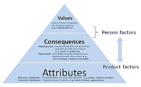


Geef een reactie
Je moet ingelogd zijn op om een reactie te plaatsen.