Tag: Statistics

  • Bivariate Analysis: Understanding Correlation, t-test, and Chi Square test

    Bivariate analysis is a statistical technique used to examine the relationship between two variables. This type of analysis is often used in fields such as psychology, economics, and sociology to study the relationship between two variables and determine if there is a significant relationship between them.

    Correlation

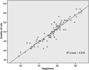
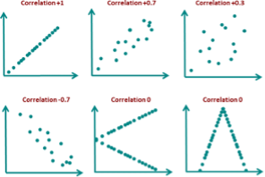
    Correlation is a measure of the strength and direction of the relationship between two variables. A positive correlation means that as one variable increases, the other variable also increases, and vice versa. A negative correlation means that as one variable increases, the other decreases. The strength of the correlation is indicated by a correlation coefficient, which ranges from -1 to +1. A coefficient of -1 indicates a perfect negative correlation, +1 indicates a perfect positive correlation, and 0 indicates no correlation.

    T-Test

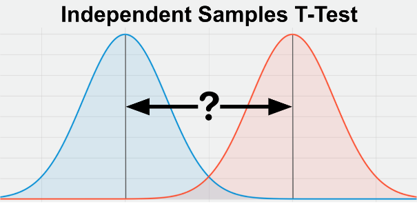
    A t-test is a statistical test that compares the means of two groups to determine if there is a significant difference between them. The t-test is commonly used to test the hypothesis that the means of two populations are equal. If the t-statistic is greater than the critical value, then the difference between the means is considered significant.

    Chi Square Test

    The chi square test is a statistical test used to determine if there is a significant association between two categorical variables. The test measures the difference between the observed frequencies and the expected frequencies in a contingency table. If the calculated chi square statistic is greater than the critical value, then the association between the two variables is considered significant.

    Significance

    Significance in statistical analysis refers to the likelihood that an observed relationship between two variables is not due to chance. In other words, it measures the probability that the relationship is real and not just a random occurrence. In statistical analysis, a relationship is considered significant if the p-value is less than a set alpha level, usually 0.05.

    In conclusion, bivariate analysis is an important tool for understanding the relationship between two variables. Correlation, t-test, and chi square test are three commonly used methods for bivariate analysis, each with its own strengths and weaknesses. It is important to understand the underlying assumptions and limitations of each method and to choose the appropriate test based on the research question and the type of data being analyzed

  • Distributions

    When working with datasets, it is important to understand the central tendency and dispersion of the data. These measures give us a general idea of how the data is distributed and what its typical values are. However, when the data is skewed or has outliers, it can be difficult to determine the central tendency and dispersion accurately. In this blog post, we’ll explore how to deal with skewed datasets and how to choose the appropriate measures of central tendency and dispersion.

    What is a Skewed Dataset?

    A skewed dataset is one in which the values are not evenly distributed. Instead, the data is skewed towards one end of the scale. There are two types of skewness: positive and negative. In a positive skewed dataset, the values are skewed to the right, while in a negative skewed dataset, the values are skewed to the left.

    Measures of Central Tendency

    Measures of central tendency are used to determine the typical value or center of a dataset. The three most commonly used measures of central tendency are the mean, median, and mode.

    1. Mean: The mean is the sum of all the values in the dataset divided by the number of values. It gives us an average value for the dataset.
    2. Median: The median is the middle value in a dataset. If the dataset has an odd number of values, the median is the value in the middle. If the dataset has an even number of values, the median is the average of the two middle values.
    3. Mode: The mode is the value that occurs most frequently in the dataset.

    In a skewed dataset, the mean is often skewed in the same direction as the data. This means that the mean may not accurately represent the typical value in a skewed dataset. In these cases, the median is often a better measure of central tendency. The median gives us the middle value in the dataset, which is not affected by outliers or skewness.

    Measures of Dispersion

    Measures of dispersion are used to determine how spread out the values in a dataset are. The two most commonly used measures of dispersion are the range and the standard deviation.

    1. Range: The range is the difference between the highest and lowest values in the dataset.
    2. Standard deviation: The standard deviation is a measure of how much the values in a dataset vary from the mean.

    In a skewed dataset, the range and standard deviation may be affected by outliers or skewness. In these cases, it is important to use other measures of dispersion, such as the interquartile range or trimmed mean, to get a more accurate representation of the dispersion in the data.

    When dealing with skewed datasets, it is important to choose the appropriate measures of central tendency and dispersion. The mean, median, and mode are measures of central tendency, while the range and standard deviation are measures of dispersion. In a skewed dataset, the mean may not accurately represent the typical value, and the range and standard deviation may be affected by outliers or skewness. In these cases, it is often better to use the median or other measures of dispersion to get a more accurate representation of the data.

  • Dependent t-test

    The dependent t-test, also known as the paired samples t-test, is a statistical method used to compare the means of two related groups, allowing researchers to assess whether significant differences exist under different conditions or over time. This test is particularly relevant in educational and psychological research, where it is often employed to analyze the impact of interventions on the same subjects. By measuring participants at two different points—such as before and after a treatment or training program—researchers can identify changes in outcomes, thus making it a valuable tool for evaluating the effectiveness of educational strategies and interventions in various contexts, including first-year university courses.

    Notably, the dependent t-test is underpinned by several key assumptions, including the requirement that the data be continuous, the observations be paired, and the differences between pairs be approximately normally distributed. Understanding these assumptions is critical, as violations can lead to inaccurate conclusions and undermine the test’s validity.

    Common applications of the dependent t-test include pre-test/post-test studies and matched sample designs, where participants are assessed on a particular variable before and after an intervention.

    Overall, the dependent t-test remains a fundamental statistical tool in academic research, with its ability to reveal insights into the effectiveness of interventions and programs. As such, mastering its application and interpretation is essential for first-year university students engaged in quantitative research methodologies.

    Assumptions When conducting a dependent t-test, it is crucial to ensure that certain assumptions are met to validate the results. Understanding these assumptions can help you identify potential issues in your data and provide alternatives if necessary.

    Assumption 1: Continuous Dependent Variable The first assumption states that the dependent variable must be measured on a continuous scale, meaning it should be at the interval or ratio level. Examples of appropriate variables include revision time (in hours), intelligence (measured using IQ scores), exam performance (scaled from 0 to 100), and weight (in kilograms).

    Assumption 2: Paired Observations The second assumption is that the data should consist of paired observations, which means each participant is measured under two different conditions. This ensures that the data is related, allowing for the analysis of differences within the same subjects.

    Assumption 3: No Significant Outliers The third assumption requires that there be no significant outliers in the differences between the paired groups. Outliers are data points that differ markedly from others and can adversely affect the results of the dependent t-test, potentially leading to invalid conclusions.

    Assumption 4: Normality of Differences The fourth assumption states that the distribution of the differences in the dependent variable should be approximately normally distributed, especially important for smaller sample sizes (N < 25)[5]. While real-world data often deviates from perfect normality, the results of a dependent t-test can still be valid if the distribution is roughly symmetric and bell-shaped.

    Common applications of the dependent t-test include pre-test/post-test studies and matched pairs designs. Scenarios for Application Repeated Measures One of the primary contexts for using the dependent t-test is in repeated measures designs. In such studies, the same subjects are measured at two different points in time or under two different conditions. For example, researchers might measure the physical performance of athletes before and after a training program, analyzing whether significant improvements occurred as a result of the intervention.

    Hypothesis Testing In conducting a dependent t-test, researchers typically formulate two hypotheses: the null hypothesis (H0) posits that there is no difference in the means of the paired groups, while the alternative hypothesis (H1) suggests that a significant difference exists. By comparing the means and calculating the test statistic, researchers can determine whether to reject or fail to reject the null hypothesis, providing insights into the effectiveness of an intervention or treatment.

  • Independent t-test

    The independent t-test, also known as the two-sample t-test or unpaired t-test, is a fundamental statistical method used to assess whether the means of two unrelated groups are significantly different from one another. This inferential test is particularly valuable in various fields, including psychology, medicine, and social sciences, as it allows researchers to draw conclusions about population parameters based on sample data when the assumptions of normality and equal variances are met. Its development can be traced back to the early 20th century, primarily attributed to William Sealy Gosset, who introduced the concept of the t-distribution to handle small sample sizes, thereby addressing limitations in traditional hypothesis testing methods. The independent t-test plays a critical role in data analysis by providing a robust framework for hypothesis testing, facilitating data-driven decision-making across disciplines. Its applicability extends to real-world scenarios, such as comparing the effectiveness of different treatments or assessing educational outcomes among diverse student groups.

    The test’s significance is underscored by its widespread usage and enduring relevance in both academic and practical applications, making it a staple tool for statisticians and researchers alike. However, the independent t-test is not without its controversies and limitations. Critics point to its reliance on key assumptions—namely, the independence of samples, normality of the underlying populations, and homogeneity of variances—as potential pitfalls that can compromise the validity of results if violated.

    Moreover, the test’s sensitivity to outliers and the implications of sample size on generalizability further complicate its application, necessitating careful consideration and potential alternative methods when these assumptions are unmet. Despite these challenges, the independent t-test remains a cornerstone of statistical analysis, instrumental in hypothesis testing and facilitating insights across various research fields. As statistical practices evolve, ongoing discussions around its assumptions and potential alternatives continue to shape its application, reflecting the dynamic nature of data analysis methodologies in contemporary research.