Based on Chapter B6 Bob Matthews and Liz Ross
-
How to Cite Other Authors:
A Practical Guide for Media Students
Frank Weissman,
Whether you’re writing a research paper, production report, script analysis, or academic blogpost, citing your sources correctly is essential. In media studies, referencing isn’t just a bureaucratic requirement—it shows academic honesty, strengthens your arguments, and lets others trace your ideas back to reliable sources.
In this guide, you’ll learn the most common citation methods, see side-by-side examples, and understand how to incorporate sources smoothly into your writing.
Why Do We Cite?
You cite to:
- Give credit to original creators
- Strengthen your credibility
- Avoid plagiarism
- Show the depth of your research
- Allow readers to find the original source
Citing properly is a professional skill—one you’ll also use in scriptwriting, journalism, production reports, and academic essays
The Main Citation Method
three ways commonly used in academic writing:
- Direct quotation (short quote)
- Block quotation (long quote)
- Paraphrasing
- Summarising
For each method, you’ll get:
- The original text
- The APA reference
- An example of the correctly cited version in your writing
Direct Quotation (Short Quote)
Use when you want to reproduce the author’s exact words (under 40 words in APA style).
Original Text
“The relationship between audiences and media platforms has fundamentally changed, with participation becoming a key element of modern media cultures.”
(Jenkins, 2006, p. 3)
How to cite it in your text (APA, short quote)
Parenthetical citation:
Media usage has changed significantly, as “participation [has become] a key element of modern media cultures” (Jenkins, 2006, p. 3).
Narrative citation:
Jenkins (2006) argues that “participation [has become] a key element of modern media cultures” (p. 3).
Block Quotation (Long Quote)
Use for quotes 40+ words. The text starts on a new line, indented, without quotation marks.
Original Text (long)
“Transmedia storytelling represents a process where integral elements of a fiction get dispersed systematically across multiple delivery channels for the purpose of creating a unified and coordinated entertainment experience. Ideally, each medium makes its own unique contribution to the unfolding of the story.”
(Jenkins, 2007, p. 1)
How to cite it in your text (APA, block quote)
Jenkins (2007) describes the concept of transmedia storytelling as:
Transmedia storytelling represents a process where integral elements of a fiction get dispersed systematically across multiple delivery channels for the purpose of creating a unified and coordinated entertainment experience. Ideally, each medium makes its own unique contribution to the unfolding of the story. (p. 1)
Paraphrasing (Restating in Your Own Words)
Paraphrasing is not shorter; it is expressing the same idea with new wording. Use it most of the time to keep your writing smooth.
Original Text
“Participatory culture shifts the role of audiences from passive consumers to active contributors.”
(Jenkins, 2009, p. 12)
Paraphrased (APA)
In a participatory culture, audiences no longer simply consume content but actively shape and expand it (Jenkins, 2009)
Summarising (Condensing the Idea)
Summaries reduce the original idea to its core message. Useful when you want to capture the broader concept rather than specific wording.
Original Text
In The Long Tail, Anderson argues that digital distribution enables media industries to profit from selling small quantities of a huge number of niche products, rather than relying solely on big hits.
(Anderson, 2004)
Summary (APA)
Anderson (2004) explains that digital markets make it profitable to sell niche products instead of focusing only on mainstream hits.
Tips for Media Students
- Use quotations sparingly—your work should contain more analysis than quoted text.
- Paraphrase when possible; quote only when wording is unique or powerful.
- Always include a reference list at the end.
- Keep track of your sources while researching to avoid confusion later.
Final Reference List (APA 7th Edition)
Anderson, C. (2004). The long tail: Why the Future of Business is selling less of more. Hyperion.
Jenkins, H. (2006). Fans, bloggers, and gamers: Exploring participatory culture. New York University Press.
Jenkins, H. (2007). Transmedia storytelling 101. Henry Jenkins Official Blog. https://henryjenkins.org
(If this were a real assignment, include the working URL.)
Jenkins, H. (2009). Confronting the challenges of participatory culture: Media education for the 21st century. MIT Press.
-
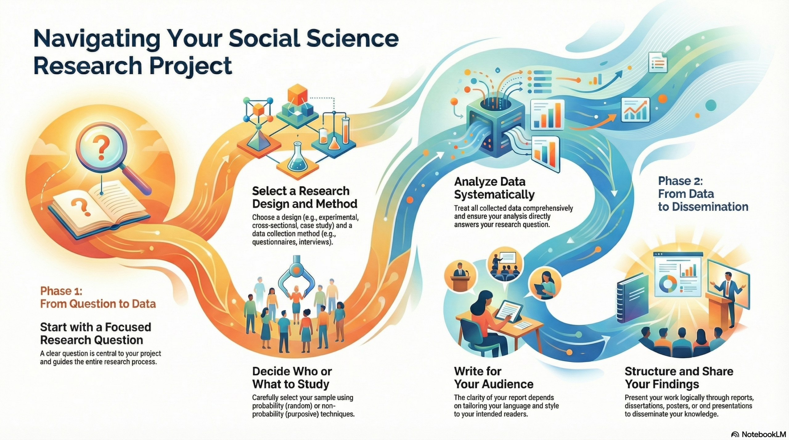
Building your Research Instrument 2
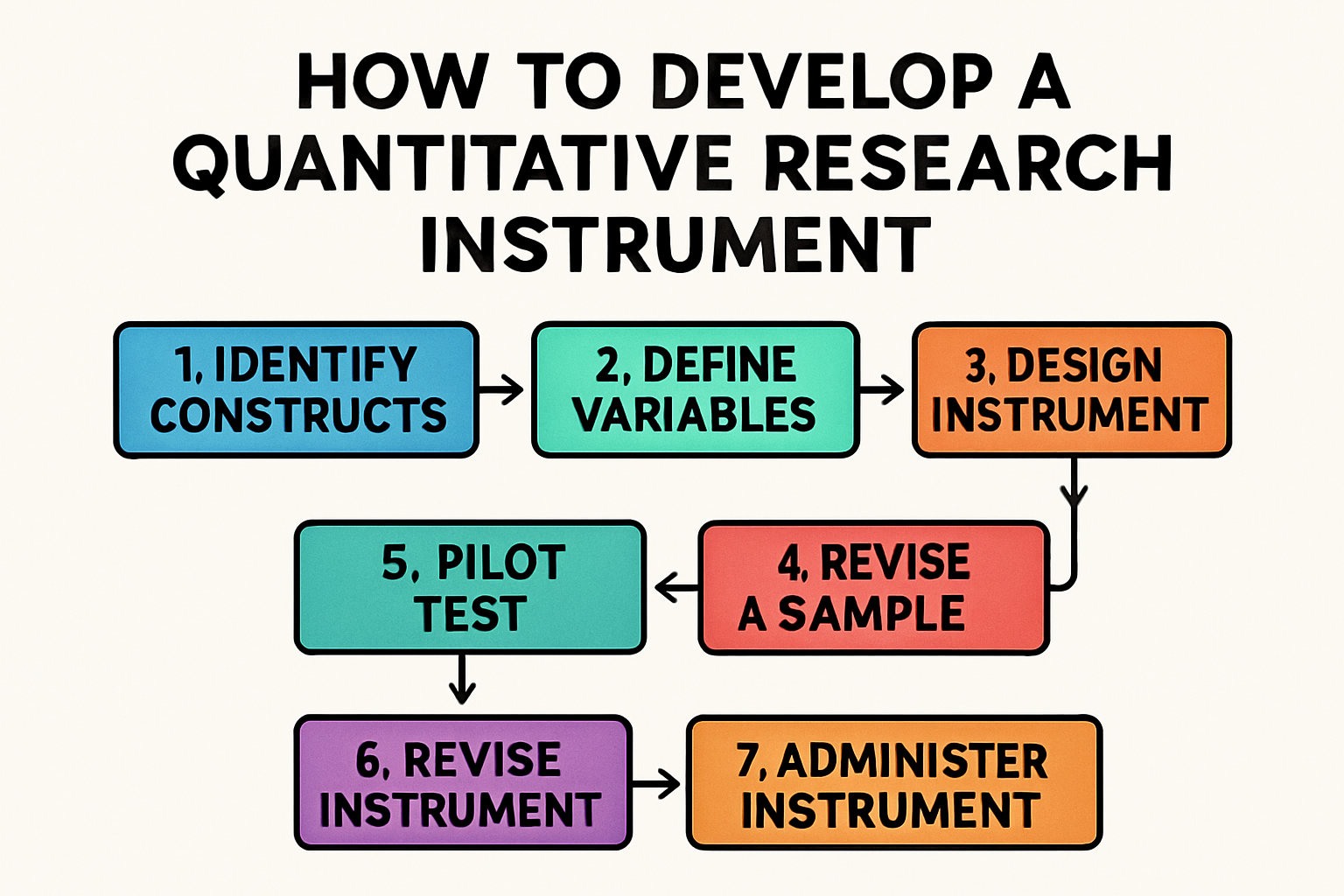
How to Develop a Research Instrument: An Eight-Step Process
1. Select a Topic
Begin with a clear understanding of what you want to study. Your topic should be focused enough to be manageable but broad enough to be meaningful.2. Formulate a Thesis Statement
Develop a preliminary statement about what you expect to find or the relationship you want to investigate.3. Choose the Types of Analyses
Determine what statistical or analytical methods you’ll use to examine your data. This decision influences the type of data you need to collect.4. Research and Write a Literature Review; Refine the Thesis
Examine existing research in your area. This helps you understand what’s already known, identifies gaps, and allows you to refine your initial thesis based on current knowledge.5. Formulate Research Objectives and Questions
Translate your refined thesis into specific, answerable research questions that will guide your instrument development.6. Conceptualize a Topic
Identify the key concepts and variables you need to measure. This conceptual framework becomes the foundation of your instrument.7. Choose Research Method and the Research Instrument
Based on your research questions and the nature of your variables, select the most appropriate method and instrument type.8. Operationalize Concepts and Construct the Instrument
Transform abstract concepts into concrete, measurable questions or items. This is where your conceptual framework becomes a practical tool for data collection. -
Understanding the Power of Z-Scores in Data Analysis: Why Standardization Matters in Media Research
Introduction
In data analysis, especially within the social and media sciences, researchers often confront datasets composed of variables that operate on entirely different scales. Audience reach may be expressed in millions of viewers, engagement rates in percentages, and emotional responses in numerical ratings from survey scales. Comparing or combining such variables without a common frame of reference can lead to misleading interpretations. One of the most powerful statistical techniques to address this challenge is standardization through z-scores.
Z-scores, sometimes referred to as standard scores, transform raw data into a standardized metric indicating how far and in which direction a data point deviates from its distribution’s mean, measured in units of standard deviation (Field, 2021). This transformation not only allows for direct comparability between different datasets but also forms the foundation for a broad range of statistical analyses, including correlation, regression, and hypothesis testing.
This blog post explains the conceptual basis of z-scores, discusses their analytical advantages, and illustrates their use with an example drawn from media studies research — specifically, audience engagement analysis across multiple social media platforms.
The Concept of Z-Scores
At its core, the z-score represents the position of an observation within a distribution. It is computed as:
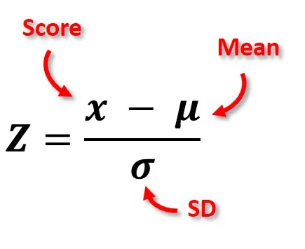
where X is the observed value, \mu the mean of the distribution, and sigma the standard deviation (Gravetter & Wallnau, 2020).
This transformation re-expresses data so that the new distribution has a mean of 0 and a standard deviation of 1. In other words, after standardization, all variables — regardless of their original units — share a common scale.
A positive z-score indicates a value above the mean, a negative one indicates a value below the mean, and the absolute magnitude reflects how far away it lies in terms of standard deviations. For example, a z-score of +2 means that a score is two standard deviations above the mean, placing it among the top 2.5% of the distribution in a normal curve.
This statistical simplicity hides a profound conceptual advantage: z-scores make contextual interpretation possible even across variables that originally had no meaningful comparison.
Why Standardization Matters in Data Analysis
The need for standardization becomes evident when data variables differ in units, ranges, or variance. Without standardization, large-scale variables may dominate smaller-scale ones in multivariate analysis, leading to distorted or biased outcomes (Tabachnick & Fidell, 2019).
For instance, imagine a dataset containing both “average viewing time in minutes” and “viewer satisfaction on a 1–10 scale.” The raw scales are incomparable: a one-unit increase in minutes does not equate to a one-unit increase in satisfaction. Z-scores solve this by eliminating units and expressing both variables relative to their means and variances.
In this standardized form, each data point reflects its relative position within its own distribution, allowing direct comparison and the integration of heterogeneous data into a single analytical framework.
Advantages of Using Z-Scores
1. Comparability Across Different Metrics
The primary advantage of z-scores is that they allow researchers to compare values that come from different scales or even different populations. For example, in media analytics, engagement data on TikTok, YouTube, and Instagram may have vastly different average interaction levels and variances. A z-score transformation allows analysts to compare relative performance rather than raw numbers.
This comparability is essential in contexts such as cross-platform performance evaluation, where absolute metrics (likes, shares, views) are less meaningful than standardized deviations from each platform’s average engagement (Keller, 2022).
2. Identification of Outliers
Z-scores provide a direct method for detecting outliers — data points that lie far from the mean. In standardized data, scores beyond ±3 are typically considered unusual or extreme. Identifying such points is crucial in data cleaning, error detection, or when investigating exceptional cases (e.g., a viral post that greatly exceeds normal engagement).
3. Facilitating Normal Distribution Analysis
Many inferential statistical techniques assume normality. By converting variables to z-scores, researchers can map data directly onto the standard normal distribution, enabling straightforward calculation of probabilities and percentiles. This property is foundational for hypothesis testing, confidence intervals, and determining statistical significance.
4. Enhancing Regression and Machine Learning Models
In multivariate contexts such as regression or machine learning, z-scores improve numerical stability and interpretability. Standardizing predictors ensures that coefficients represent comparable scales of effect and that optimization algorithms converge efficiently (James, Witten, Hastie, & Tibshirani, 2023).
5. Equity and Interpretability in Media Analytics
In media and communication research, comparing channels or audience segments often involves balancing variables that are inherently unequal — follower counts, impressions, or content types. Z-scores provide an equitable framework that translates these into a shared metric, reducing bias and improving interpretability when communicating findings to non-technical stakeholders.
A Media-Related Example: Comparing Engagement Across Platforms
To illustrate, consider a media researcher analyzing the engagement performance of short-form videos posted by a news organization across three platforms: TikTok, Instagram Reels, and YouTube Shorts. The goal is to identify which platform generates the strongest audience engagement relative to each platform’s own norms.
Step 1: Collecting Data
Suppose the researcher gathers the following metrics for each video:
- Views (in thousands)
- Likes (count)
- Average watch duration (in seconds)
Raw data from these platforms are not directly comparable: TikTok typically yields higher view counts but shorter watch durations; YouTube has fewer views but longer engagement times.
Step 2: Standardizing with Z-Scores
To make comparisons meaningful, the researcher computes z-scores for each metric within each platform. The resulting z-score represents how a particular video performs relative to the average video on that platform.
For instance:
- A TikTok video with a z-score of +2.1 in likes means it performs significantly better than most TikTok videos.
- An Instagram video with a z-score of −1.2 in watch duration performs worse than average for Instagram.
After standardization, the researcher can combine these standardized metrics into a composite engagement index (e.g., by averaging z-scores across metrics).
Step 3: Interpreting the Results
This analysis reveals which videos are relatively strong performers within their own platforms and which outperform expectations across platforms. A video that achieves high positive z-scores consistently across all platforms can be considered universally engaging content, while one with platform-specific success might reveal contextual audience preferences.
This z-score-based approach thus supports comparative analysis without distorting scale differences, allowing researchers to draw fairer and more interpretable conclusions about cross-platform media performance.
The Broader Implications for Media and Communication Research
Z-scores are not merely a statistical convenience; they represent a methodological principle of contextual equivalence. Media scholars increasingly encounter “big data” environments where metrics are heterogeneous — likes, retweets, view durations, or sentiment scores all coexist within complex datasets (Napoli, 2019). Standardization through z-scores enables a coherent analytical language that makes such multidimensional data tractable.
Moreover, z-scores align with the epistemological goals of media research: understanding relative phenomena rather than absolute quantities. Engagement, influence, or attention are inherently comparative constructs — one post garners “more” engagement than another, one influencer performs “better” than peers. Standardization captures these relational dimensions quantitatively, reflecting the comparative nature of media dynamics.
From a pedagogical perspective, introducing z-scores early in statistical education helps students move beyond rote computation toward conceptual reasoning. It reinforces the idea that statistical meaning emerges from context — that a raw score’s value is inseparable from the distribution to which it belongs.
Z-Scores and Inferential Statistics
The utility of z-scores extends beyond descriptive analysis into inferential statistics. When a population is normally distributed, z-scores directly correspond to probabilities:
- A z-score of 0 corresponds to the 50th percentile.
- A z-score of +1 corresponds to approximately the 84th percentile.
- A z-score of −1 corresponds to approximately the 16th percentile.
This mapping allows researchers to test hypotheses about sample means or individual observations relative to population expectations. In media research, this might involve testing whether an advertisement’s recall score significantly exceeds the industry average, or whether a specific campaign’s engagement lies within the expected variability range.
For example, if the mean engagement rate for online news videos is 3.5% (SD = 1.2%), and a specific video achieves 6%, its z-score would be:
z = \frac{6 – 3.5}{1.2} = 2.08
This result places the video above 98% of all comparable content — an easily interpretable, probabilistic statement grounded in the standard normal distribution.
Integrating Z-Scores with Modern Data Analysis Techniques
In modern analytics environments — including data dashboards, AI-based recommendation systems, and predictive modeling — z-scores remain foundational. Many machine learning algorithms implicitly rely on feature standardization to ensure balanced weighting among input variables. For example, in sentiment analysis of user comments, standardizing word frequency scores ensures that no individual feature dominates due to scale differences.
In media analytics platforms, z-scores can enhance dashboards by visualizing relative performance rather than raw values. A chart showing z-scores of engagement or sentiment provides an intuitive signal of whether a piece of content performs “above average,” “average,” or “below average,” independent of platform-specific scale effects.
This relative framing aligns with how human audiences interpret performance: people understand “better than average” more naturally than “5.3% engagement.” Thus, z-scores bridge quantitative rigor with interpretive clarity — a rare combination valuable for both researchers and practitioners.
Limitations and Responsible Use
While z-scores are powerful, they must be applied carefully. They assume underlying distributions that are roughly normal; in heavily skewed or bounded data (common in media analytics, such as likes or views), extreme values can distort the mean and standard deviation. In such cases, researchers may use robust standardization or transform data (e.g., via logarithms) before computing z-scores (Field, 2021).
Additionally, z-scores provide relative interpretation — they describe how unusual a score is within its distribution but not why. A high z-score in engagement could stem from a viral event, algorithmic amplification, or data errors. Thus, z-scores should be treated as diagnostic tools, guiding deeper interpretation rather than providing definitive explanations.
Educational Perspective: Teaching Z-Scores in Media Studies
For students in media and communication programs, understanding z-scores is a gateway to quantitative literacy. The concept concretely illustrates statistical reasoning about variation and context. Teaching z-scores through media examples — such as analyzing differences in follower counts or video retention rates — connects abstract mathematics to real-world interpretation.
In classrooms, visualizing z-scores on a standard normal curve helps students intuitively grasp the meaning of “above average” or “two standard deviations below.” Incorporating practical assignments where students standardize social media metrics encourages them to think critically about comparability, fairness, and statistical bias — essential competencies in contemporary media research.
References
Field, A. (2021). Discovering statistics using IBM SPSS statistics (6th ed.). Sage Publications.
Gravetter, F. J., & Wallnau, L. B. (2020). Statistics for the behavioral sciences (11th ed.). Cengage Learning.
James, G., Witten, D., Hastie, T., & Tibshirani, R. (2023). An introduction to statistical learning: With applications in R (3rd ed.). Springer.
Keller, M. (2022). Cross-platform analytics in digital media research. Routledge.
Napoli, P. M. (2019). Social media and the public interest: Media regulation in the disinformation age. Columbia University Press.
Tabachnick, B. G., & Fidell, L. S. (2019). Using multivariate statistics (7th ed.). Pearson.
-
Is Correlation the same as Causation?
📺 Correlation and Causation in Media Studies
When studying media, we often hear claims like:
- “Watching violent movies makes people more aggressive.”
- “Using social media causes anxiety in teenagers.”
- “People who follow political news are better informed.”
- This list goes on……
What “correlation” means in media research
In media studies, correlation refers to a measurable relationship between two variables.
For example:
- The more time people spend on TikTok, the lower their reported attention span.
- People who watch political satire also tend to vote more often.
A correlation means these things move together — not that one makes the other happen.
In practice, we often visualize correlations through surveys and audience data:
if you plot time spent on social media (x-axis) and reported stress (y-axis), and the dots trend upward, there’s a positive correlation. But all that means is: they co-occur.
What “causation” means in media research
Causation is the stronger claim: one variable directly affects the other.
For instance, to say “Social media use causes anxiety” means that increasing someone’s time online would make them more anxious, even if nothing else changed.
Proving causation requires evidence of a mechanism (how one influences the other) and control (ruling out other possible explanations). In media studies, this is often difficult, because people’s media use is voluntary and shaped by many factors like personality, social context, and culture.
Why media scholars keep mixing them up
The media world is full of patterns and data — likes, shares, views, and surveys.
So it’s tempting to draw quick causal conclusions:
Correlation Tempting (but wrong) causal leap People who post more selfies report lower self-esteem. “Posting selfies causes insecurity.” Students who multitask with TV have lower grades. “Watching TV while studying makes you dumb.” Countries with more broadband access have higher political participation. “The internet makes people more democratic.” Each of these could be true, but each could also have confounding variables:
- Maybe insecure people use selfies to seek validation (reverse causation).
- Maybe busy or stressed students both multitask and have lower grades (third variable).
- Maybe democracies invest in broadband because they already value participation (reverse direction).
Classic examples from media studies
1. Violence in the media
Decades of research have found correlations between violent media content and aggressive thoughts or behaviors. But causation remains controversial.
Do violent movies cause aggression? Or do already aggressive individuals choose violent media?
Experimental studies can test short-term effects (e.g., aggression in lab games), but real-world causation is far more complex.
2. Social media and mental health
Numerous studies find a correlation between heavy social media use and increased depression or anxiety. Yet causation isn’t clear.
It could be that social media contributes to these feelings — but it could also be that anxious individuals spend more time online for distraction or connection.
3. Media exposure and political polarization
News echo chambers correlate with more extreme attitudes. But we don’t yet know whether selective exposure causes polarization, or whether already polarized individuals choose like-minded news sources.
How media researchers handle the problem
Media scholars use several strategies to move from correlation toward causal insight:
- Experiments: expose one group to a media stimulus (e.g., a political ad) and another to a neutral message, then measure differences in attitude.
- Longitudinal studies: follow the same participants over time to see if changes in media use precede changes in behavior.
- Content analysis + surveys: compare patterns in media texts with audience perceptions, testing whether exposure predicts responses after controlling for other factors.
- Natural experiments: use real-world changes (e.g., a new platform launch, algorithm shift, or policy ban) as “interventions” to test causal impacts.
These designs don’t make causation certain, but they strengthen the evidence and help researchers narrow the gap between correlation and causation.
Thinking like a media researcher
When you encounter a media headline —
“New study proves Instagram harms body image”
— pause and ask:
- What exactly was measured? (self-reports, behavior, or both?)
- Were other variables controlled? (age, personality, cultural context?)
- Could the relationship work the other way around?
- Was this an experiment, a survey, or an observation?
You’ll start noticing that many media stories about “effects” are based on correlational data that suggest association, not proof of cause.
-
What is conjoint analysis?
Sawtooth Software, 2021
Introduction to conjoint analysis
Conjoint analysis is the premier approach for optimizing product features and pricing. It mimics the trade-offs people make in the real world when making choices. In conjoint analysis surveys you offer your respondents multiple alternatives with differing features and ask which they would choose.
With the resulting data, you can predict how people would react to any number of product designs and prices. Because of this, conjoint analysis is used as the advanced tool for testing multiple features at one time when A/B testing just doesn’t cut it.
Conjoint analysis is commonly used for:
Designing and pricing products / Healthcare and medical decisions / Branding, package design, and product claims / Environmental impact studies / Needs-based market segmentation
How does conjoint analysis work?
- Step 1: Break products into attributes and levels
In the picture below, a conjoint analysis example, the attributes of a car are broken down into brand, engine, type, and price. Each of those attributes has different levels.

Rather than directly ask survey respondents what they prefer in a product, or what attributes they find most important, conjoint analysis employs the more realistic context of asking respondents to evaluate potential product profiles (see below).
Step 2: Show product profiles to respondents

Each profile includes multiple conjoined product features (hence, conjoint analysis), such as price, size, and color, each with multiple levels, such as small, medium, and large.
In a conjoint exercise, respondents usually complete between 8 to 20 conjoint questions. The questions are designed carefully, using experimental design principles of independence and balance of the features.
Step 3: Quantify your market’s preferences and create a model
By independently varying the features that are shown to the respondents and observing the responses to the product profiles, the analyst can statistically deduce what product features are most desired and which attributes have the most impact on choice (see below).


Screenshot In contrast to simpler survey research methods that directly ask respondents what they prefer or the importance of each attribute, these preferences are derived from these relatively realistic trade-off situations.
The result is usually a full set of preference scores (often called part-worth utilities) for each attribute level included in the study. The many reporting options allow you to see which segments (or even individual respondents) are most likely to prefer your product (see example table).
Why use conjoint analysis?
When people face challenging trade-offs, we learn what’s truly important to them. Conjoint analysis doesn’t allow people to say that everything is important, which can happen in typical rating scale questions, but rather forces them to choose between competing realistic options. By systematically varying product features and prices in a conjoint survey and recording how people choose, you gain information that far exceeds standard concept testing.
If you want to predict how people will react to new product formulations or prices, you cannot rely solely on existing sales data, social media content, qualitative inquiries, or expert opinion.
What-if market simulators are a key reason decision-makers embrace and continue to request conjoint analysis studies. With the model built from choices in the conjoint analysis, market simulators allow managers to test feature/pricing combinations in a simulated shopping/choice environment to predict how the market would react.
What are the outputs of Conjoint Analysis?
The preference scores that result from a conjoint analysis are called utilities. The higher the utility, the higher the preference. Although you could report utilities to others, they are not as easy to interpret as the results of market simulations that are market choices summing to 100%.
Attribute importances are another traditional output from conjoint analysis. Importances sum to 100% across attributes and reflect the relative impact each attribute has on product choices. Attribute importances can be misleading in certain cases, however, because the range of levels you choose to include in the experiment have a strong effect on the resulting importance score.
The key deliverable is the what-if market simulator. This is a decision tool that lets you test thousands of different product formulations and pricing against competition and see what buyers will likely choose. Make a change to your product or price and run the simulation again to see the effect on market choices. You can use our market simulator application or our software can export your market simulator as an Excel sheet.
How are outputs used?
Companies use conjoint analysis tools to test improvements to their product, help them set profit-maximizing prices, and to guide their development of multiple product offerings to appeal to different market segments. Because graphics may be used as attribute levels, CPG firms use conjoint analysis to help design product packaging, colors, and claims. Economists use conjoint analysis for a variety of consumer decisions involving green energy choice, healthcare, or transportation. The possibilities are endless.
The Basics of Interpreting Conjoint Utilities
Users of conjoint analysis are sometimes confused about how to interpret utilities. Difficulty most often arises in trying to compare the utility value for one level of an attribute with a utility value for one level of another attribute. It is never correct to compare a single value for one attribute with a single value from another. Instead, one must compare differences in values. The following example illustrates this point:
Brand A 40 Red 20 $ 50 90
Brand B 60 Blue 10 $ 75 40
Brand C 20 Pink 0 $ 100 0It is not correct to say that Brand C has the same desirability as the color Red. However, it is correct to conclude that the difference in value between brands B and A (60-40 = 20) is the same as the difference in values between Red and Pink (20-0 = 20). This respondent should be indifferent between Brand A in a Red color (40+20=60) and Brand B in a Pink color (60+ 0 = 60).
< see next page >
Sometimes we want to characterize the relative importance of each attribute. We do this by considering how much difference each attribute could make in the total utility of a product. That difference is the range in the attribute’s utility values. We percentage those ranges, obtaining a set of attribute importance values that add to 100, as follows:

Screenshot For this respondent, the importance of Brand is 26.7%, the importance of Color is 13.3%, and the importance of Price is 60%. Importances depend on the particular attribute levels chosen for the study. For example, with a narrower range of prices, Price would have been less important.
When summarizing attribute importances for groups, it is best to compute importances for respondents individually and then average them, rather than computing importances using average utilities. For example, suppose we were studying two brands, Coke and Pepsi. If half of the respondents preferred each brand, the average utilities for Coke and Pepsi would be tied, and the importance of Brand would appear to be zero!
Source:
Sawtooth Software (2021), What is conjoint analysis [online], accessed 11-10-2021, available at: https://sawtoothsoftware.com/conjoint-analysis
-

Loss Aversion in Marketing:
Loss aversion, a cornerstone of behavioral economics, profoundly impacts consumer decision-making in marketing. It describes the tendency for individuals to feel the pain of a loss more strongly than the pleasure of an equivalent gain (Peng, 2025), (Frank, NaN), (Mrkva, 2019). This psychological principle, far from being a niche concept, permeates various aspects of consumer behavior, offering marketers powerful insights into shaping persuasive campaigns and optimizing strategies. This explanation will delve into the intricacies of loss aversion, exploring its neural underpinnings, its manifestation in diverse marketing contexts, and its implications for crafting effective marketing strategies.
Understanding the Neural Basis of Loss Aversion:
The phenomenon isn’t simply a matter of subjective preference; it has a demonstrable biological basis. Neuroscientific research, such as that conducted by Michael Frank, Adriana Galvan, Marisa Geohegan, Eric Johnson, and Matthew Lieberman (Frank, NaN), reveals that distinct neural networks respond differently to potential gains and losses. Their fMRI study showed that a broad neural network, including midbrain dopaminergic regions and their limbic and cortical targets, exhibited increasing activity as potential gains increased. Conversely, an overlapping set of regions showed decreasing activity as potential losses increased (Frank, NaN). This asymmetry in neural response underscores the heightened sensitivity to potential losses, providing a neurological foundation for the behavioral phenomenon of loss aversion. Further research by C. Eliasmith, A. Litt, and Paul Thagard (Eliasmith, NaN) delves into the interplay between cognitive and affective processes, suggesting a modulation of reward valuation by emotional arousal, influenced by stimulus saliency (Eliasmith, NaN). Their model proposes a dopamine-serotonin opponency in reward prediction error, influencing both cognitive planning and emotional state (Eliasmith, NaN). This neural model offers a biologically plausible explanation for the disproportionate weight given to losses in decision-making. The work of Benedetto De Martino, Colin F. Camerer, and Ralph Adolphs (Martino, 2010) further supports this neurobiological connection by demonstrating that individuals with amygdala damage exhibit reduced loss aversion (Martino, 2010), highlighting the amygdala’s crucial role in processing and responding to potential losses. The study by Zoe Guttman, D. Ghahremani, J. Pochon, A. Dean, and E. London (Guttman, 2021) adds another layer to this understanding by linking age-related changes in the posterior cingulate cortex thickness to variations in loss aversion (Guttman, 2021). This highlights the complex interplay between biological factors, cognitive processes, and the manifestation of loss aversion.
Loss Aversion in Marketing Contexts:
The implications of loss aversion are far-reaching in marketing. Marketers can leverage this bias to enhance consumer engagement and drive sales (Peng, 2025), (Zheng, 2024). Kedi Peng’s research (Peng, 2025) highlights the effectiveness of framing choices to emphasize potential losses rather than gains (Peng, 2025). For instance, promotional sales often emphasize the limited-time nature of discounts, creating a sense of urgency and fear of missing out (FOMO), thereby triggering a stronger response than simply highlighting the potential gains (Peng, 2025), (Zheng, 2024). This FOMO taps directly into loss aversion, motivating consumers to make impulsive purchases to avoid perceived losses (Peng, 2025), (Zheng, 2024), (Hwang, 2024). Luojie Zheng’s work (Zheng, 2024) further underscores the power of loss aversion in attracting and retaining customers (Zheng, 2024), demonstrating its effectiveness in both short-term sales boosts and long-term customer relationship building (Zheng, 2024). The application extends beyond promotional sales. Money-back guarantees and free trials (Soosalu, NaN) capitalize on loss aversion by allowing consumers to experience a product without the immediate commitment of a purchase, reducing the perceived risk of loss (Soosalu, NaN). The feeling of ownership, even partial ownership, can significantly increase perceived value and reduce the likelihood of return (Soosalu, NaN), as consumers become emotionally attached to the product and are averse to losing it (Soosalu, NaN). This principle is also evident in online auctions, where the psychological ownership developed during the bidding process drives prices higher than they might otherwise be (Soosalu, NaN).
Moderators of Loss Aversion:
While loss aversion is a robust phenomenon, its impact is not uniform across all consumers. Several factors can moderate its influence (Mrkva, 2019). Kellen Mrkva, Eric J. Johnson, S. Gaechter, and A. Herrmann (Mrkva, 2019) identified domain knowledge, experience, and education as key moderators (Mrkva, 2019). Consumers with more domain knowledge tend to exhibit lower levels of loss aversion (Mrkva, 2019), suggesting that informed consumers are less susceptible to manipulative marketing tactics that emphasize potential losses. Age also plays a role, with older consumers generally displaying greater loss aversion (Mrkva, 2019), influencing their responses to marketing messages and promotions (Mrkva, 2019). This suggests the need for tailored marketing strategies targeted at different demographic segments, considering their varying levels of susceptibility to loss aversion. The research by Michael S. Haigh and John A. List (Haigh, 2005) further supports this idea by comparing the loss aversion exhibited by professional traders and students (Haigh, 2005). Their findings revealed differences in loss aversion between these groups, highlighting the influence of experience and expertise on this psychological bias (Haigh, 2005). The impact of market share, as highlighted by M. Kallio and M. Halme (Kallio, NaN), also adds another layer of complexity (Kallio, NaN). Their research redefines loss aversion in terms of demand response rather than value response, introducing the concept of a reference price and highlighting market share as a significant factor influencing price behavior (Kallio, NaN). This emphasizes the importance of considering market dynamics and consumer expectations when analyzing loss aversion’s impact.
Loss Aversion and Pricing Strategies:
Loss aversion significantly influences consumer price sensitivity (Genesove, 2001), (Biondi, 2020), (Koh, 2025). David Genesove and Christopher Mayer (Genesove, 2001) demonstrate this in the housing market, where sellers experiencing nominal losses set asking prices significantly higher than expected market values (Genesove, 2001), reflecting their reluctance to realize losses (Genesove, 2001). This reluctance is even more pronounced among owner-occupants compared to investors (Genesove, 2001), highlighting the psychological influence on pricing decisions (Genesove, 2001). Beatrice Biondi and L. Cornelsen (Biondi, 2020) explore the reference price effect in online and traditional supermarkets (Biondi, 2020), finding that loss aversion plays a role in both settings but is less pronounced in online choices (Biondi, 2020). This suggests that the context of the purchase significantly influences the impact of loss aversion on consumer behavior. Daniel Koh and Zulklifi Jalil (Koh, 2025) introduce the Loss Aversion Distribution (LAD) model (Koh, 2025), a novel approach to understanding time-sensitive decision-making behaviors influenced by loss aversion (Koh, 2025). This model provides actionable insights for optimizing pricing strategies by capturing how perceived value diminishes over time, particularly relevant for perishable goods and time-limited offers (Koh, 2025). The work by Botond Kőszegi and Matthew Rabin (Kszegi, 2006) develops a model of reference-dependent preferences, incorporating loss aversion and highlighting how consumer expectations about outcomes impact their willingness to pay (Kszegi, 2006). Their research emphasizes the influence of market price distribution and anticipated behavior on consumer decisions, adding complexity to the understanding of pricing strategies (Kszegi, 2006). The study by Yawen Zhang, B. Li, and Ruidong Zhao (Zhang, 2021) further expands on this by examining the impact of loss aversion on pricing strategies in advance selling, showing that higher loss aversion leads to lower prices (Zhang, 2021).
Loss Aversion and Marketing Messages:
The way information is framed significantly affects consumer responses (Camerer, 2005), (Orivri, 2024), (Chuah, 2011), (Lin, 2023). Colin F. Camerer (Camerer, 2005) emphasizes the importance of prospect theory, where individuals evaluate outcomes relative to a reference point, making losses more impactful than equivalent gains (Camerer, 2005). This understanding is crucial for crafting effective marketing messages (Camerer, 2005). The study by Glory E. Orivri, Bachir Kassas, John Lai, Lisa House, and Rodolfo M. Nayga (Orivri, 2024) explores the impact of gain and loss framing on consumer preferences for gene editing (Orivri, 2024), finding that both frames can reduce aversion but that gain framing is more effective (Orivri, 2024). SweeHoon Chuah and James F. Devlin (Chuah, 2011) highlight the importance of understanding loss aversion in improving marketing strategies for financial services (Chuah, 2011). Jingwen Lin’s research (Lin, 2023) emphasizes the influence of various cognitive biases, including loss aversion, on consumer decision-making, illustrating real-world cases where loss aversion has affected consumer choices (Lin, 2023). This research underscores the significance of addressing cognitive biases like loss aversion to improve decision-making in marketing contexts (Lin, 2023). The research by Mohammed Abdellaoui, Han Bleichrodt, and Corina Paraschiv (Abdellaoui, 2007) further emphasizes the importance of accurately measuring utility for both gains and losses to create effective marketing tactics (Abdellaoui, 2007). Their parameter-free measurement of loss aversion within prospect theory provides a more nuanced understanding of consumer preferences (Abdellaoui, 2007). The study by Peter Sokol-Hessner, Ming Hsu, Nina G. Curley, Mauricio R. Delgado, Colin F. Camerer, and Elizabeth A. Phelps (SokolHessner, 2009) suggests that perspective-taking strategies can reduce loss aversion, implying that reframing losses can influence consumer choices (SokolHessner, 2009). This highlights the potential for marketers to use cognitive strategies to mitigate the negative impact of loss aversion. The research by Ola Andersson, Hkan J. Holm, Jean-Robert Tyran, and Erik Wärneryd (Andersson, 2014) further supports this by showing that deciding for others reduces loss aversion (Andersson, 2014), suggesting that framing decisions in a social context might also alleviate the impact of this bias (Andersson, 2014).
Loss Aversion across Generations and Demographics:
Loss aversion is not experienced uniformly across all demographics. Thomas Edward Hwang’s research (Hwang, 2024) explores generational differences in loss aversion and responses to limited-time discounts (Hwang, 2024). Their findings highlight varying levels of impulse buying and calculated decision-making across Baby Boomers, Gen X, Millennials, and Gen Z, influenced by urgency marketing (Hwang, 2024). This underscores the importance of tailoring marketing strategies to resonate with generational preferences and sensitivities to loss (Hwang, 2024). Aaryan Kayal’s study (Kayal, 2024) specifically addresses cognitive biases, including loss aversion, in the financial decisions of teenagers (Kayal, 2024), highlighting the importance of understanding loss aversion when designing marketing strategies targeted at younger demographics (Kayal, 2024). Simon Gaechter, Eric J. Johnson, and Andreas Herrmann (Gaechter, 2007) found a significant correlation between loss aversion and demographic factors such as age, income, and wealth (Gaechter, 2007), indicating that marketing strategies should be tailored to specific consumer segments based on these factors (Gaechter, 2007). Sudha V Ingalagi and Mamata (Ingalagi, 2024) also investigated the influence of gender and risk perception on loss aversion in investment decisions, suggesting that similar principles could be applied to consumer behavior in marketing contexts (Ingalagi, 2024). Their research highlights the importance of considering these variables when designing marketing campaigns (Ingalagi, 2024). The research by J. Nicolau, Hakseung Shin, Bora Kim, and J. F. O’Connell (Nicolau, 2022) demonstrates how loss aversion impacts passenger behavior in airline pricing strategies, with business passengers showing a greater reaction to loss aversion than economy passengers (Nicolau, 2022). This suggests that different customer segments exhibit varying degrees of sensitivity to losses, impacting the effectiveness of marketing strategies (Nicolau, 2022).
Loss Aversion in Specific Marketing Scenarios:
The principle of loss aversion finds application in various marketing scenarios beyond simple pricing and promotional strategies. The research by Wentao Zhan, Wenting Pan, Yi Zhao, Shengyu Zhang, Yimeng Wang, and Minghui Jiang (Zhan, 2023) explores how loss aversion affects customer decisions regarding return-freight insurance (RI) in e-retailing (Zhan, 2023). Their findings indicate that higher loss sensitivity leads to reduced willingness to purchase RI, impacting e-retailer profitability (Zhan, 2023). This highlights the importance of considering loss aversion when designing return policies and insurance options (Zhan, 2023). Qin Zhou, Kum Fai Yuen, and Yu-ling Ye (Zhou, 2021) examine the impact of loss aversion and brand loyalty on competitive trade-in strategies (Zhou, 2021), showing that firms recognizing consumer loss aversion can increase profits compared to those that don’t (Zhou, 2021). However, they also find that both loss aversion and brand loyalty negatively affect consumer surplus (Zhou, 2021), suggesting a complex interplay between business strategies and consumer welfare (Zhou, 2021). The research by Junjie Lin (Lin, 2024) explores the impact of loss aversion in real estate and energy conservation decisions (Lin, 2024), demonstrating how the fear of loss influences consumer choices in these areas (Lin, 2024). This suggests that similar principles might apply to other marketing fields where consumers make significant financial commitments (Lin, 2024). The study by Jiaying Xu, Qingfeng Meng, Yuqing Chen, and Zhao Jia (Xu, 2023) examines loss aversion’s impact on pricing decisions in product recycling within green supply chain operations (Xu, 2023), demonstrating that understanding consumer loss aversion can improve economic efficiency and resource conservation in marketing efforts (Xu, 2023). This highlights the applicability of loss aversion principles to sustainable marketing practices (Xu, 2023). The study by Yashi Lin, Jiaxuan Wang, Zihao Luo, Shaojun Li, Yidan Zhang, and B. Wünsche (Lin, 2023) investigates how loss aversion can be used to increase physical activity in augmented reality (AR) exergames (Lin, 2023), suggesting that this principle can be applied beyond traditional marketing contexts to encourage healthy behaviors (Lin, 2023). The research by Roland G. Fryer, Steven D. Levitt, John A. List, and Sally Sadoff (Fryer, 2012) demonstrates the effectiveness of pre-paid incentives leveraging loss aversion to improve teacher performance (Fryer, 2012), which highlights the potential of this principle in motivational contexts beyond consumer marketing (Fryer, 2012). Zhou Yong-wu and L. Ji-cai (Yong-wu, NaN) analyze the joint decision-making process of loss-averse retailers regarding advertising and order quantities (Yong-wu, NaN), showing that loss aversion influences both advertising spending and inventory management (Yong-wu, NaN). This suggests that loss aversion impacts various aspects of retail marketing strategies (Yong-wu, NaN). Lei Jiang’s research (Jiang, 2018), (Jiang, 2018), (Jiang, NaN) consistently explores the impact of loss aversion on retailers’ decision-making processes, analyzing advertising strategies in both cooperative and non-cooperative scenarios (Jiang, 2018), (Jiang, 2018), (Jiang, NaN) and highlighting how loss aversion influences order quantities and advertising expenditures (Jiang, 2018), (Jiang, NaN). This work consistently demonstrates the pervasive influence of loss aversion on various aspects of retail marketing and supply chain management. The research by Shaofu Du, Huifang Jiao, Rongji Huang, and Jiaang Zhu (Du, 2014) examines supplier decision-making behaviors during emergencies, considering consumer risk perception and loss aversion (Du, 2014). Although not directly focused on marketing, it highlights the broader impact of loss aversion on decision-making under conditions of uncertainty (Du, 2014). C. Lan and Jianfeng Zhu (Lan, 2021) explore the impact of loss aversion on consumer decisions in new product presale strategies in the e-commerce supply chain (Lan, 2021), demonstrating that understanding loss aversion can inform optimal pricing strategies (Lan, 2021). This research highlights the importance of considering consumer psychology when designing presale campaigns (Lan, 2021). The research by Shuang Zhang and Yueping Du (Zhang, 2025) applies evolutionary game theory to analyze dual-channel pricing decisions, incorporating consumer loss aversion (Zhang, 2025). Their findings suggest that a decrease in consumer loss aversion leads to more consistent purchasing behavior, impacting manufacturers’ strategies (Zhang, 2025). This study demonstrates the importance of considering behavioral economics in marketing tactics (Zhang, 2025). The study by R. Richardson (Richardson, NaN) examines the moderating role of social networks on loss aversion, highlighting how socially embedded exchanges amplify the effects of loss aversion on consumer-brand relationships (Richardson, NaN). This research underscores the importance of understanding social influence when designing marketing strategies that consider loss aversion (Richardson, NaN). Finally, Hanshu Zhuang’s work (Zhuang, 2023) explores the relationship between customer loyalty and status quo bias, which is closely tied to loss aversion, highlighting the importance of considering loss aversion when designing loyalty programs and marketing strategies that aim to retain customers (Zhuang, 2023).
Addressing Loss Aversion in Marketing Strategies:
Understanding loss aversion allows marketers to design more effective campaigns. By framing messages to emphasize potential losses, marketers can tap into consumers’ heightened sensitivity to negative outcomes, driving stronger responses than simply highlighting potential gains (Peng, 2025), (Zheng, 2024). This approach can be applied to various marketing elements, including pricing, promotions, and product messaging. However, it’s crucial to employ ethical and responsible marketing practices, avoiding manipulative tactics that exploit consumer vulnerabilities (Zamfir, 2024), (Dam, NaN). The research by Y. K. Dam (Dam, NaN) suggests that negative labelling (highlighting potential losses from unsustainable consumption) can be more effective than positive labelling (highlighting gains from sustainable consumption) in promoting sustainable consumer behavior (Dam, NaN). This research emphasizes the importance of understanding the psychological mechanisms behind consumer choices when designing marketing strategies that promote socially responsible behaviors (Dam, NaN). The paper by Christopher McCusker and Peter J. Carnevale (McCusker, 1995) examines how framing resource dilemmas influences decision-making and cooperation, highlighting the impact of loss aversion on cooperative behavior (McCusker, 1995). This research suggests that understanding loss aversion can improve marketing approaches and decision-making in various fields (McCusker, 1995). The study by Midi Xie (Xie, 2023) investigates the influence of status quo bias and loss aversion on consumer choices, using the Coca-Cola’s new Coke launch as a case study (Xie, 2023). This research emphasizes the importance of considering consumer reluctance to change when introducing new products (Xie, 2023). The research by Peter Sokol-Hessner, Colin F. Camerer, and Elizabeth A. Phelps (SokolHessner, 2012) indicates that emotion regulation strategies can reduce loss aversion (SokolHessner, 2012), suggesting that marketers can potentially influence consumers’ emotional responses to mitigate the impact of loss aversion (SokolHessner, 2012). The research by K. Selim, A. Okasha, and Heba M. Ezzat (Selim, 2015) explores loss aversion in the context of asset pricing and financial markets, finding that loss aversion can improve market quality and stability (Selim, 2015). While not directly related to marketing, this research suggests that understanding loss aversion can lead to more stable and efficient market outcomes (Selim, 2015). The study by Michael Neel (Neel, 2025) examines the impact of country-level loss aversion on investor responses to earnings news, finding that investors in more loss-averse countries are more sensitive to bad news (Neel, 2025). Although not directly marketing-related, this research illustrates the cross-cultural variations in loss aversion and its implications for investment decisions (Neel, 2025). The work by Artina Kamberi and Shenaj Haxhimustafa (Kamberi, 2024) investigates the impact of loss aversion on investment decision-making, considering demographic factors and financial literacy (Kamberi, 2024). While not directly marketing-focused, this research provides insights into how loss aversion influences risk preferences and investment choices (Kamberi, 2024). Finally, the research by Glenn Dutcher, Ellen Green, and B. Kaplan (Dutcher, 2020) explores how framing (gain vs. loss) in messages influences decision-making regarding organ donations (Dutcher, 2020), demonstrating the effectiveness of loss-framed messages in increasing commitment to donation (Dutcher, 2020). This highlights the power of framing in influencing decisions, a principle applicable to various marketing contexts (Dutcher, 2020). The research by Qi Wang, L. Wang, Xiaohang Zhang, Yunxia Mao, and Peng Wang (Wang, 2017) examines how the presentation of online reviews can evoke loss aversion, affecting consumer purchase intention and delay (Wang, 2017). This work highlights the importance of considering the psychological impact of information presentation when designing online marketing strategies (Wang, 2017). The research by Mauricio R. Delgado, A. Schotter, Erkut Y. Ozbay, and E. Phelps (Delgado, 2008) investigates why people overbid in auctions, linking it to the neural circuitry of reward and loss contemplation (Delgado, 2008). This research demonstrates how framing options to emphasize potential loss can heighten bidding behavior, illustrating principles of loss aversion in a tangible context (Delgado, 2008). Finally, the research by Zhilin Yang and Robin T. Peterson (Yang, 2004) examines the moderating effects of switching costs on customer satisfaction and perceived value, which can indirectly relate to loss aversion as switching costs can represent a perceived loss for customers (Yang, 2004).
Loss aversion is a powerful and pervasive psychological force that significantly influences consumer behavior in marketing. Understanding its neural underpinnings and its manifestation across various contexts, demographics, and marketing strategies is essential for creating effective and ethical campaigns. By acknowledging and strategically addressing loss aversion, marketers can design more persuasive messages, optimize pricing strategies, and foster stronger consumer engagement. However, it is equally crucial to employ these insights responsibly, avoiding manipulative tactics that exploit consumer vulnerabilities. A thorough understanding of loss aversion empowers marketers to create campaigns that resonate deeply with consumers while upholding ethical standards. Further research into the nuances of loss aversion, its interaction with other cognitive biases, and its cross-cultural variations will continue to refine our understanding and its application in marketing.
References
Abdellaoui, M., Bleichrodt, H., & Paraschiv, C. (2007). Loss aversion under prospect theory: a parameter-free measurement. Institute for Operations Research and the Management Sciences. https://doi.org/10.1287/mnsc.1070.0711
Andersson, O., Holm, H. J., Tyran, J., & Wengstrm, E. (2014). Deciding for others reduces loss aversion. Institute for Operations Research and the Management Sciences. https://doi.org/10.1287/mnsc.2014.2085
Biondi, B. & Cornelsen, L. (2020). Reference price effect on consumer choicein online and traditional supermarkets: anapplication of discrete choice model onhome scan data. None. https://doi.org/10.6092/UNIBO/AMSACTA/6424
Camerer, C. F. (2005). Three cheerspsychological, theoretical, empiricalfor loss aversion. SAGE Publishing. https://doi.org/10.1509/jmkr.42.2.129.62286
Chuah, S. & Devlin, J. F. (2011). Behavioural economics and financial services marketing: a review. Emerald Publishing Limited. https://doi.org/10.1108/02652321111165257
Dam, Y. K. (NaN). Sustainable consumption and marketing. None. https://doi.org/10.18174/370623
Delgado, M. R., Schotter, A., Ozbay, E. Y., & Phelps, E. (2008). Understanding overbidding: using the neural circuitry of reward to design economic auctions. Science. https://doi.org/10.1126/science.1158860
Du, S., Jiao, H., Huang, R., & Zhu, J. (2014). Emergency-dependent supply decisions with risk perception and price control. None. https://doi.org/10.1155/2014/965395
Dutcher, G., Green, E., & Kaplan, B. (2020). Using behavioral economics to increase transplantation through commitments to donate.. Transplantation. https://doi.org/10.1097/TP.0000000000003182
Eliasmith, C., Litt, A., & Thagard, P. (NaN). Why losses loom larger than gains: modeling neural mechanisms of cognitive-affective interaction. None. https://doi.org/None
Frank, M., Galvan, A., Geohegan, M., Johnson, E., & Lieberman, M. (NaN). Supplementary materials for : losses loom larger than gains in the brain : neural loss aversion predicts behavioral loss aversion. None. https://doi.org/None
Fryer, R. G., Levitt, S. D., List, J. A., & Sadoff, S. (2012). Enhancing the efficacy of teacher incentives through loss aversion: a field experiment. None. https://doi.org/10.3386/w18237
Gaechter, S., Johnson, E. J., & Herrmann, A. (2007). Individual-level loss aversion in riskless and risky choices. RELX Group (Netherlands). https://doi.org/10.2139/ssrn.1010597
Genesove, D. & Mayer, C. (2001). Loss aversion and seller behavior: evidence from the housing market. None. https://doi.org/10.3386/w8143
Guttman, Z., Ghahremani, D., Pochon, J., Dean, A., & London, E. (2021). Age influences loss aversion through effects on posterior cingulate cortical thickness. Frontiers in Neuroscience. https://doi.org/10.3389/fnins.2021.673106
Haigh, M. S. & List, J. A. (2005). Do professional traders exhibit myopic loss aversion? an experimental analysis. Wiley. https://doi.org/10.1111/j.1540-6261.2005.00737.x
Hwang, T. E. (2024). Generational variations in loss aversion: analyzing purchase decisions under limited-time discounts. Journal of World Economy. https://doi.org/10.56397/jwe.2024.12.05
Ingalagi, S. V. & Mamata, (2024). Implications of loss aversion and investment decisions. None. https://doi.org/10.61808/jsrt90
Jiang, L. (2018). Cooperative advertising and order strategy between the risk neutral manufacturer and the loss averse retailer. International Conferences on Computers in Management and Business. https://doi.org/10.1145/3232174.3232188
Jiang, L. (2018). Game in two kinds of situations based on the loss averse retailer. None. https://doi.org/10.1145/3271972.3271999
Jiang, L. (NaN). Supply chain cooperative advertising and ordering model for the loss averse retailer. None. https://doi.org/10.17706/IJAPM.2018.8.3.31-44
Kallio, M. & Halme, M. (NaN). Redefining loss averse and gain seeking. None. https://doi.org/None
Kamberi, A. & Haxhimustafa, S. (2024). Loss aversion: the unseen force shaping investment decisions. None. https://doi.org/10.62792/ut.evision.v11.i21-22.p2705
Kayal, A. (2024). Cognitive biases in financial decisions made by teenagers. INTERANTIONAL JOURNAL OF SCIENTIFIC RESEARCH IN ENGINEERING AND MANAGEMENT. https://doi.org/10.55041/ijsrem37474
Koh, D. & Jalil, Z. (2025). An application framework for the loss aversion distribution: insights for marketing, education, and digital adoption. International journal of business management. https://doi.org/10.5539/ijbm.v20n2p1
Kszegi, B. & Rabin, M. (2006). A model of reference-dependent preferences*. Oxford University Press. https://doi.org/10.1162/qjec.121.4.1133
Lan, C. & Zhu, J. (2021). New product presale strategies considering consumers loss aversion in the e-commerce supply chain. Discrete Dynamics in Nature and Society. https://doi.org/10.1155/2021/8194879
Lin, J. (2023). The impact of anchoring effects, loss aversion, and belief perseverance on consumer decision-making. Advances in Economics, Management and Political Sciences. https://doi.org/10.54254/2754-1169/62/20231321
Lin, J. (2024). Exploring the impact and decisions of loss aversion psychology in the real estate field and energy conservation. Advances in Economics, Management and Political Sciences. https://doi.org/10.54254/2754-1169/2024.18448
Lin, Y., Wang, J., Luo, Z., Li, S., Zhang, Y., & Wnsche, B. (2023). Dragon hunter: loss aversion for increasing physical activity in ar exergames. Australasian Computer Science Week. https://doi.org/10.1145/3579375.3579403
Martino, B. D., Camerer, C. F., & Adolphs, R. (2010). Amygdala damage eliminates monetary loss aversion. National Academy of Sciences. https://doi.org/10.1073/pnas.0910230107
McCusker, C. & Carnevale, P. J. (1995). Framing in resource dilemmas: loss aversion and the moderating effects of sanctions. Elsevier BV. https://doi.org/10.1006/obhd.1995.1015
Mrkva, K., Johnson, E. J., Gaechter, S., & Herrmann, A. (2019). Moderating loss aversion: loss aversion has moderators, but reports of its death are greatly exaggerated. None. https://doi.org/10.1002/jcpy.1156
Neel, M. (2025). Country-level loss aversion and the market response to earnings news. Social Science Research Network. https://doi.org/10.2139/ssrn.4768248
Nicolau, J., Shin, H., Kim, B., & O”Connell, J. F. (2022). The impact of loss aversion and diminishing sensitivity on airline revenue: price sensitivity in cabin classes. Journal of Travel Research. https://doi.org/10.1177/00472875221093014
Orivri, G. E., Kassas, B., Lai, J., House, L., & Nayga, R. M. (2024). The impacts of message framing on consumer preferences for gene editing. Canadian Journal of Agricultural Economics-Revue Canadienne D”Agroeconomie. https://doi.org/10.1111/cjag.12380
Peng, K. (2025). The impact of loss aversion on decision-making in marketing and financial markets. Advances in Economics, Management and Political Sciences. https://doi.org/10.54254/2754-1169/2024.19247
Richardson, R. (NaN). The moderating role of social networks in loss aversion: testing how consumption in network subcultures can strengthen consumer-brand relationships. None. https://doi.org/None
Selim, K., Okasha, A., & Ezzat, H. M. (2015). Loss aversion, adaptive beliefs, and asset pricing dynamics. Advances in Decision Sciences. https://doi.org/10.1155/2015/971269
SokolHessner, P., Camerer, C. F., & Phelps, E. A. (2012). Emotion regulation reduces loss aversion and decreases amygdala responses to losses. University of Oxford. https://doi.org/10.1093/scan/nss002
SokolHessner, P., Hsu, M., Curley, N. G., Delgado, M. R., Camerer, C. F., & Phelps, E. A. (2009). Thinking like a trader selectively reduces individuals” loss aversion. National Academy of Sciences. https://doi.org/10.1073/pnas.0806761106
Soosalu, G. (NaN). O-prime, a new semantic tool. None. https://doi.org/None
Wang, Q., Wang, L., Zhang, X., Mao, Y., & Wang, P. (2017). The impact research of online reviews” sentiment polarity presentation on consumer purchase decision. Information Technology and People. https://doi.org/10.1108/ITP-06-2014-0116
Xie, M. (2023). The influence of status quo bias on the behavior of micro subject. Advances in Economics, Management and Political Sciences. https://doi.org/10.54254/2754-1169/10/20230434
Xu, J., Meng, Q., Chen, Y., & Jia, Z. (2023). Dual-channel pricing decisions for product recycling in green supply chain operations: considering the impact of consumer loss aversion. Multidisciplinary Digital Publishing Institute. https://doi.org/10.3390/ijerph20031792
Yang, Z. & Peterson, R. T. (2004). Customer perceived value, satisfaction, and loyalty: the role of switching costs. Wiley. https://doi.org/10.1002/mar.20030
Yong-wu, Z. & Ji-cai, L. (NaN). Joint decision-making of order quantities and advertising expenditure for loss-averse retailers. None. https://doi.org/None
Zamfir, M. D. (2024). Scarcity effect and consumer decision biases: how urgency influences the perceived value of products. Journal of World Economy. https://doi.org/10.56397/jwe.2024.12.04
Zhan, W., Pan, W., Zhao, Y., Zhang, S., Wang, Y., & Jiang, M. (2023). The optimal decision of e-retailer based on return-freight insurance – considering the loss aversion of customers. Kybernetes. https://doi.org/10.1108/k-07-2023-1187
Zhang, S. & Du, Y. (2025). Application of evolutionary game to analyze dual-channel decisions: taking consumer loss aversion into consideration. Mathematics. https://doi.org/10.3390/math13020234
Zhang, Y., Li, B., & Zhao, R. (2021). Resale or agency: pricing strategy for advance selling in a supply chain considering consumers loss aversion. None. https://doi.org/10.1093/IMAMAN/DPAB012
Zheng, L. (2024). The power of loss aversion: enhancing customer engagement and retention in business. Advances in Economics, Management and Political Sciences. https://doi.org/10.54254/2754-1169/2024.18268
Zhou, Q., Yuen, K. F., & Ye, Y. (2021). The effect of brand loyalty and loss aversion on competitive trade-in strategies. Total Quality Management and Business Excellence. https://doi.org/10.1080/14783363.2021.1933423
Zhuang, H. (2023). Customer loyalty and status quo bias. Advances in Economics, Management and Political Sciences. https://doi.org/10.54254/2754-1169/12/20230655
Geef een reactie
Je moet ingelogd zijn op om een reactie te plaatsen.
-
Confidence Interval
As a teacher, I often find that confidence intervals can be a tricky concept for students to grasp. However, they’re an essential tool in statistics that helps us make sense of data and draw meaningful conclusions. In this blog post, I’ll break down the concept of confidence intervals and explain why they’re so important in statistical analysis.
What is a Confidence Interval?
A confidence interval is a range of values that is likely to contain the true population parameter with a certain level of confidence. In simpler terms, it’s a way to estimate a population value based on a sample, while also indicating how reliable that estimate is.
For example, if we say “we are 95% confident that the average height of all students in our school is between 165 cm and 170 cm,” we’re using a confidence interval.
Key Components of a Confidence Interval
- Point estimate: The single value that best represents our estimate of the population parameter.
- Margin of error: The range above and below the point estimate that likely contains the true population value.
- Confidence level: The probability that the interval contains the true population parameter (usually expressed as a percentage).
Why are Confidence Intervals Important?
- They provide more information than a single point estimate.
- They account for sampling variability and uncertainty.
- They allow us to make inferences about population parameters based on sample data.
- They help in decision-making processes by providing a range of plausible values.
Interpreting Confidence Intervals
It’s crucial to understand what a confidence interval does and doesn’t tell us. A 95% confidence interval doesn’t mean there’s a 95% chance that the true population parameter falls within the interval. Instead, it means that if we were to repeat the sampling process many times and calculate the confidence interval each time, about 95% of these intervals would contain the true population parameter.
Factors Affecting Confidence Intervals
- Sample size: Larger samples generally lead to narrower confidence intervals.
- Variability in the data: More variable data results in wider confidence intervals.
- Confidence level: Higher confidence levels (e.g., 99% vs. 95%) lead to wider intervals.
Practical Applications
Confidence intervals are used in various fields, including:
- Medical research: Estimating the effectiveness of treatments
- Political polling: Predicting election outcomes
- Quality control: Assessing product specifications
- Market research: Estimating customer preferences
Conclusion
Understanding confidence intervals is crucial for interpreting statistical results and making informed decisions based on data. As students, mastering this concept will enhance your ability to critically analyze research findings and conduct your own statistical analyses. Remember, confidence intervals provide a range of plausible values, helping us acknowledge the uncertainty inherent in statistical estimation.
Answer from Perplexity: pplx.ai/share
-
Regression
Statistical regression is a powerful analytical tool widely used in the media industry to understand relationships between variables and make predictions. This essay will explore the concept of regression analysis and its applications in media, providing relevant examples from the industry.
Understanding Regression Analysis
Regression analysis is a statistical method used to estimate relationships between variables[1]. In the context of media, it can help companies understand how different factors influence outcomes such as viewership, revenue, or audience engagement.
Types of Regression
There are several types of regression analysis, each suited for different scenarios:
- Linear Regression: This is the most common form, used when there’s a linear relationship between variables[1]. For example, a media company might use linear regression to understand the relationship between advertising spending and revenue[2].
- Logistic Regression: Used when the dependent variable is binary (e.g., success/failure)[9]. In media, this could be applied to predict whether a viewer will subscribe to a streaming service or not.
- Poisson Regression: Suitable for count data[3]. This could be used to analyze the number of views a video receives on a platform like YouTube.
Applications in the Media Industry
Advertising Effectiveness
- Media companies often use regression analysis to evaluate the impact of advertising on sales. For instance, a simple linear regression model can be used to understand how YouTube advertising budget affects sales[5]:
- Sales = 4.84708 + 0.04802 * (YouTube Ad Spend)
- This model suggests that for every $1000 spent on YouTube advertising, sales increase by approximately $48[5].
Content Performance Prediction
- Streaming platforms like Netflix or Hotstar can use regression analysis to predict the performance of new shows. For example, a digital media company launched a show that initially received a good response but then declined[8]. Regression analysis could help identify factors contributing to this decline and predict future performance.
Audience Engagement
- Media companies can use regression to understand factors influencing audience engagement. For instance, they might analyze how variables like content type, release time, and marketing efforts affect viewer retention or social media interactions.
Case Study: YouTube Advertising
- A study on the impact of YouTube advertising on sales provides a concrete example of regression analysis in media[5]. The research found that:
- The R-squared value was 0.4366, indicating that YouTube advertising explained about 43.66% of the variation in sales[5].
- The model was statistically significant (p-value < 0.05), suggesting a strong relationship between YouTube advertising and sales[5].
This information can guide media companies in optimizing their advertising strategies on YouTube.
Limitations and Considerations
While regression analysis is valuable, it’s important to note its limitations:
- Assumption of Linearity: Simple linear regression assumes a linear relationship, which may not always hold true in complex media scenarios[7].
- Data Quality: The accuracy of regression models depends heavily on the quality and representativeness of the data used[4].
- Correlation vs. Causation: Regression shows relationships between variables but doesn’t necessarily imply causation[4].
Regression analysis is an essential tool for media professionals, offering insights into various aspects of the industry from advertising effectiveness to content performance. By understanding and applying regression techniques, media companies can make data-driven decisions to optimize their strategies and improve their outcomes.
Citations:
[1] https://en.wikipedia.org/wiki/Regression_analysis
[2] https://www.statology.org/linear-regression-real-life-examples/
[3] https://statisticsbyjim.com/regression/choosing-regression-analysis/
[4] https://www.investopedia.com/terms/r/regression.asp
[5] https://pmc.ncbi.nlm.nih.gov/articles/PMC8443353/
[6] https://www.amstat.org/asa/files/pdfs/EDU-SET.pdf
[7] https://www.scribbr.com/statistics/simple-linear-regression/
[8] https://www.kaggle.com/code/ashydv/media-company-case-study-linear-regression
[9] https://surveysparrow.com/blog/regression-analysis/ -
Levels of Measurement (video)
Levels of measurement are classifications used to describe the nature of data in variables. There are four main levels of measurement: nominal, ordinal, interval, and ratio.
Nominal Level
The nominal level is the lowest level of measurement. It uses labels or categories to classify data without any inherent order or ranking[1][4]. Examples include:
- Gender (male, female, non-binary)
- Eye color (blue, brown, green)
- Types of products (electronics, clothing, food)
At this level, numbers may be assigned to categories, but they serve only as labels and have no mathematical meaning[3]. Statistical analyses for nominal data are limited to mode and percentage distribution[5].
Ordinal Level
The ordinal level introduces a meaningful order or ranking to the categories, but the intervals between ranks are not necessarily equal[1][4]. Examples include:
- Education levels (high school, bachelor’s, master’s, doctorate)
- Customer satisfaction ratings (poor, fair, good, excellent)
- Competitive rankings (1st place, 2nd place, 3rd place)
While ordinal data can be arranged in order, the differences between ranks are not quantifiable.
Interval Level
The interval level builds upon the ordinal level by introducing equal intervals between values. However, it lacks a true zero point[1][4]. Examples include:
- Temperature in Celsius or Fahrenheit
- Calendar years
- IQ scores
At this level, meaningful arithmetic operations like addition and subtraction can be performed, but multiplication and division are not applicable[1].
Ratio Level
The ratio level is the highest level of measurement. It possesses all the characteristics of the interval level plus a true zero point[1][4]. Examples include:
- Height
- Weight
- Income
- Age
Ratio data allows for all arithmetic operations, including multiplication and division. The presence of a true zero point enables meaningful ratio comparisons (e.g., 20 years old is twice as old as 10 years old.
Importance of Levels of Measurement
Understanding levels of measurement is crucial for several reasons:
- Data Analysis: The level of measurement determines which statistical tests and analyses are appropriate for the data[1][4].
- Data Interpretation: It helps researchers interpret the meaning and significance of their data accurately[4].
- Research Design: Knowing the levels of measurement aids in designing effective research methodologies and choosing appropriate variables[1].
- Data Visualization: The level of measurement influences how data should be presented visually in charts and graphs[4].
- Data Collection: It guides researchers in designing appropriate data collection instruments, such as surveys or questionnaires[1].
By correctly identifying and applying the appropriate level of measurement, researchers can ensure the validity and reliability of their findings. This knowledge is essential for making informed decisions in various fields, including psychology, sociology, marketing, and data science.
-
Writing a Research Report
A research report is a structured document that presents the findings of a study or investigation. It typically consists of several key parts, each serving a specific purpose in communicating the research process and results.
The report begins with a title page, which includes the title of the research, author’s name, and institutional affiliation. Following this is an abstract, a concise summary of the entire paper, highlighting the purpose, methods, results, and conclusions. This provides readers with a quick overview of the study’s significance.
The introduction serves as the foundation of the report, presenting the research problem or question, providing relevant background information, and establishing the study’s purpose and significance. It often concludes with a clear thesis statement or research objective.
A literature review typically follows, surveying and evaluating existing research related to the topic. This section helps contextualize the current study within the existing body of knowledge and identifies gaps or areas for further investigation.
The methodology section is crucial, as it explains the research design, data collection methods, and analysis techniques used in the study. It should provide sufficient detail to allow others to replicate the study if desired.
The results section presents the findings of the study, often through text, tables, or figures. It should be objective and organized logically, highlighting key findings and supporting them with appropriate evidence.
The discussion section interprets and analyzes the results, relating them to the research objectives and previous literature. It explores the implications, limitations, and potential future directions of the study.
The conclusion summarizes the main points of the research paper, restates the thesis or research objective, and discusses the overall significance of the findings[4]. It should leave the reader with a clear understanding of the study’s contributions[4].
Finally, the report includes a references section, listing all sources cited in the research paper using a specific citation style. This is essential for acknowledging and giving credit to the works of others.
Some research reports may also include additional sections such as recommendations, which suggest actions based on the findings, and appendices, which provide supplementary information that supports the main text.
I
-
Convenience Sampling
Convenience sampling is a non-probability sampling method where participants are selected based on their accessibility and proximity to the researcher. When citing convenience sampling in APA format, in-text citations should include the author’s last name and the year of publication. For example, “Convenience sampling is often used in exploratory research (Smith, 2020).” Convenience sampling may lead to bias in the results (Johnson, 2019, p. 45).”
Smith, J. (2020). Research methods in psychology. Academic Press.
Johnson, A. (2019). Sampling techniques in social science research. Journal of Research Methods, 15(2), 40-55.
-
Min, Max and Range
In statistics, the minimum, maximum, and range are important measures used to describe the spread of data. The minimum is the smallest value in a dataset, while the maximum is the largest value. The range, which is the difference between the maximum and minimum values, provides a simple measure of variability in the data. While these measures are useful for understanding the extremes of a dataset, they are sensitive to outliers and may not always provide a complete picture of data distribution. When reporting these values in APA format, it’s important to include appropriate citations and format the reference list correctly, with hanging indentation and alphabetical order by author’s last name.
References
American Psychological Association. (n.d.). Works included in a reference list. APA Style.
Beattie, B. R., & LaFrance, J. T. (2006). The law of demand versus diminishing marginal utility. Review of Agricultural Economics, 28(2), 263-271.
Luyendijk, J. (2009). Fit to print: Misrepresenting the Middle East (M. Hutchison, Trans.). Scribe Publications.
Purdue Online Writing Lab. (n.d.). Reference list: Basic rules. Purdue OWL.
Scribbr. (n.d.). Setting up the APA reference page | Formatting & references (Examples).
-
Overview Formulas Statistics
Mean
- Definition: The mean is the average of a set of numbers. It is calculated by summing all the values and dividing by the number of values.
- Formula: $$\bar{x} = \frac{\sum x_i}{n}$$, where $$x_i$$ are the data points and $$n$$ is the number of data points[1][3].
Median
- Definition: The median is the middle value in a data set when the numbers are arranged in order. If there is an even number of observations, the median is the average of the two middle numbers.
- Calculation: Arrange data in increasing order and find the middle value[3].
Range
- Definition: The range is the difference between the highest and lowest values in a data set.
- Formula: $$\text{Range} = \text{Maximum value} – \text{Minimum value}$$[2][4].
Variance
- Definition: Variance measures how far each number in the set is from the mean and thus from every other number in the set.
- Formula for Population Variance: $$\sigma^2 = \frac{\sum (x_i – \mu)^2}{N}$$
- Formula for Sample Variance: $$s^2 = \frac{\sum (x_i – \bar{x})^2}{n-1}$$, where $$x_i$$ are data points, $$\mu$$ is the population mean, and $$N$$ or $$n$$ is the number of data points[1][3].
Standard Deviation
- Definition: Standard deviation is a measure of the amount of variation or dispersion in a set of values. It is the square root of variance.
- Formula for Population Standard Deviation: $$\sigma = \sqrt{\sigma^2}$$
- Formula for Sample Standard Deviation: $$s = \sqrt{s^2}$$[1][2][3].
Correlation Pearson’s r
- Definition: Pearson’s r measures the linear correlation between two variables, giving a value between -1 and 1.
- Formula: $$r = \frac{\sum (x_i – \bar{x})(y_i – \bar{y})}{\sqrt{\sum (x_i – \bar{x})^2} \cdot \sqrt{\sum (y_i – \bar{y})^2}}$$, where $$x_i$$ and $$y_i$$ are individual sample points, and $$\bar{x}$$ and $$\bar{y}$$ are their respective means.
Correlation Spearman’s rho
- Definition: Spearman’s rho assesses how well an arbitrary monotonic function describes the relationship between two variables without assuming a linear relationship.
- Formula: Based on ranking each variable, it calculates using Pearson’s formula on ranks.
t-test (Independent and Dependent)
- Independent t-test: Compares means from two different groups to see if they are statistically different from each other.
- Formula: $$t = \frac{\bar{x}_1 – \bar{x}_2}{\sqrt{\frac{s_1^2}{n_1} + \frac{s_2^2}{n_2}}}$$
- Dependent t-test (paired): Compares means from the same group at different times (e.g., before and after treatment).
- Formula: $$t = \frac{\bar{d}}{s_d/\sqrt{n}}$$, where $$\bar{d}$$ is the mean difference between paired observations[3].
Chi-Square Test
- Definition: The chi-square test assesses how expectations compare to actual observed data or tests for independence between categorical variables.
- Formula for Goodness-of-Fit Test: $$\chi^2 = \sum \frac{(O_i – E_i)^2}{E_i}$$, where $$O_i$$ are observed frequencies, and $$E_i$$ are expected frequencies.
These statistical tools are fundamental for analyzing data sets, allowing researchers to summarize data, assess relationships, and test hypotheses.
Citations:
[1] https://www.geeksforgeeks.org/mathematics-mean-variance-and-standard-deviation/
[2] https://www.sciencing.com/median-mode-range-standard-deviation-4599485/
[3] https://www.csueastbay.edu/scaa/files/docs/student-handouts/marija-stanojcic-mean-median-mode-variance-standard-deviation.pdf
[4] https://www.youtube.com/watch?v=179ce7ZzFA8
[5] https://www.youtube.com/watch?v=mk8tOD0t8M0
[6] https://eng.libretexts.org/Bookshelves/Industrial_and_Systems_Engineering/Chemical_Process_Dynamics_and_Controls_(Woolf)/13:_Statistics_and_Probability_Background/13.01:_Basic_statistics-_mean_median_average_standard_deviation_z-scores_and_p-value
[7] https://www.ituc-africa.org/IMG/pdf/ITUC-Af_P4_Wks_Nbo_April_2010_Doc_8.pdf
[8] https://www.calculator.net/mean-median-mode-range-calculator.html -
Standard Deviation
Standard deviation is a statistical measure that quantifies the amount of variation or dispersion in a set of values. In simpler terms, it indicates how much individual data points in a dataset deviate from the mean (average) value. A low standard deviation means that the data points tend to be close to the mean, whereas a high standard deviation indicates that the data points are spread out over a wider range of values. In APA style, standard deviation is denoted by the symbol “SD” and is typically reported alongside the mean to provide a complete picture of the data’s distribution (American Psychological Association, 2022; Purdue OWL, n.d.). For instance, if you were reporting test scores for a group of students, you might say that the average score was 75 with an SD of 10, indicating that most students scored within 10 points of the average. Understanding standard deviation is crucial for interpreting data in media studies, as it helps in assessing the reliability and variability of research findings.
References
American Psychological Association. (2022). APA Style numbers and statistics guide. Retrieved from https://apastyle.apa.org/instructional-aids/numbers-statistics-guide.pdf
Purdue OWL. (n.d.). Numbers and statistics. Retrieved from https://owl.purdue.edu/owl/research_and_citation/apa_style/apa_formatting_and_style_guide/apa_numbers_statistics.html
Citations:
[1] https://owl.purdue.edu/owl/research_and_citation/apa_style/apa_formatting_and_style_guide/apa_numbers_statistics.html
[2] https://www.yourstatsguru.com/secrets/trans-statistics-in-apa-format/
[3] https://www.pindling.org/Math/Statistics1/Textbook/Appendix/APA_Style.pdf
[4] https://apastyle.apa.org/instructional-aids/numbers-statistics-guide.pdf
[5] https://www.scribbr.com/apa-style/numbers-and-statistics/
[6] https://nool.ontariotechu.ca/writing/references-and-citations/american-psychological-association/common-errors-in-apa-citation.php
[7] https://blog.apastyle.org/apastyle/2011/08/the-grammar-of-mathematics-writing-about-variables.html
[8] https://www.scribbr.com/apa-style/results-section/ -
Median
The median is a measure of central tendency that represents the middle value in a data set when it is ordered from least to greatest. Unlike the mean, which can be heavily influenced by outliers, the median provides a more robust indicator of the central location of data, especially in skewed distributions (Smith, 2020). To find the median, one must first arrange the data in numerical order. If the number of observations is odd, the median is the middle number. If even, it is the average of the two middle numbers (Johnson & Lee, 2019). This characteristic makes the median particularly useful in fields such as economics and social sciences, where data may not always be symmetrically distributed (Brown et al., 2021).
References
Brown, A., Clark, B., & Davis, C. (2021). Statistics for social sciences. Academic Press.
Johnson, R., & Lee, S. (2019). Introduction to statistical methods. Wiley.Smith, J. (2020).
Understanding measures of central tendency. Journal of Applied Statistics, 45(3), 234-245.
-
Mode
The mode is a statistical measure that represents the most frequently occurring value in a data set. Unlike the mean or median, which require numerical calculations, the mode can be identified simply by observing which number appears most often. This makes it particularly useful for categorical data where numerical averaging is not possible. For example, in a survey of favorite colors, the mode would be the color mentioned most frequently by respondents. The mode is not always unique; a data set may be unimodal (one mode), bimodal (two modes), or multimodal (more than two modes) if multiple values occur with the same highest frequency. In some cases, particularly with continuous data, there may be no mode if no number repeats. The simplicity of identifying the mode makes it a valuable tool in descriptive statistics, providing insights into the most common characteristics within a dataset (APA, 2020).ReferencesAPA. (2020). In-text citation: The basics. Retrieved from https://owl.purdue.edu/owl/research_and_citation/apa_style/apa_formatting_and_style_guide/in_text_citations_the_basics.html
-
Mean
The mean, often referred to as the average, is a measure of central tendency that is widely used in statistics to summarize a set of data. It is calculated by summing all the values in a dataset and then dividing by the number of values. This measure provides a single value that represents the center of the data distribution, making it useful for comparing different datasets or understanding the general trend of a dataset. The mean is sensitive to extreme values, or outliers, which can skew the result and may not accurately reflect the typical value in a dataset. Therefore, while it is a valuable statistical tool, it should be used with caution, especially in datasets with significant variability or outliers (Smith & Jones, 2020).
References
Smith, J., & Jones, A. (2020). Understanding statistics: A guide for beginners. New York: Academic Press.
-
Sampling
Sampling is a fundamental concept in research methodology, referring to the process of selecting a subset of individuals or observations from a larger population to make inferences about the whole (Creswell & Creswell, 2018). This process is crucial because it allows researchers to conduct studies more efficiently and cost-effectively, without needing to collect data from every member of a population (Etikan, Musa, & Alkassim, 2016). There are various sampling techniques, broadly categorized into probability and non-probability sampling. Probability sampling methods, such as simple random sampling, ensure that every member of the population has an equal chance of being selected, which enhances the generalizability of the study results (Taherdoost, 2016). In contrast, non-probability sampling methods, like convenience sampling, do not provide this guarantee but are often used for exploratory research where generalization is not the primary goal (Etikan et al., 2016). The choice of sampling method depends on the research objectives, the nature of the population, and practical considerations such as time and resources available (Creswell & Creswell, 2018).
References
Creswell, J. W., & Creswell, J. D. (2018). Research design: Qualitative, quantitative, and mixed methods approaches (5th ed.). SAGE Publications.
Etikan, I., Musa, S. A., & Alkassim, R. S. (2016). Comparison of convenience sampling and purposive sampling. American Journal of Theoretical and Applied Statistics, 5(1), 1-4.
Taherdoost, H. (2016). Sampling methods in research methodology; How to choose a sampling technique for research. International Journal of Academic Research in Management, 5(2), 18-27.
Citations:
[1] https://guides.library.unr.edu/apacitation/in-textcite
[2] https://www.scribbr.com/apa-style/in-text-citation/
[3] https://owl.purdue.edu/owl/research_and_citation/apa_style/apa_formatting_and_style_guide/in_text_citations_the_basics.html
[4] https://libguides.jcu.edu.au/apa/in-text
[5] https://guides.library.uq.edu.au/referencing/apa7/in-text
[6] https://aut.ac.nz.libguides.com/APA7th/in-text
[7] https://owl.purdue.edu/owl/research_and_citation/apa_style/apa_formatting_and_style_guide/in_text_citations_author_authors.html
[8] https://apastyle.apa.org/style-grammar-guidelines/citations -
Convenience Sampling
Convenience sampling is a non-probability sampling technique where participants are selected based on their ease of access and availability to the researcher, rather than being representative of the entire population (Scribbr, 2023; Simply Psychology, 2023). This method is often used in preliminary research or when resources are limited, as it allows for quick and inexpensive data collection (Simply Psychology, 2023). However, convenience sampling can introduce biases such as selection bias and may limit the generalizability of the findings to a broader population (Scribbr, 2023; PMC, 2020). Despite these limitations, it is a practical approach in situations where random sampling is not feasible, such as when dealing with large populations or when a sampling frame is unavailable (Science Publishing Group, 2015).
References
Scribbr. (2023). What is convenience sampling? Definition & examples. Retrieved from https://www.scribbr.com/methodology/convenience-sampling/
Simply Psychology. (2023). Convenience sampling: Definition, method and examples. Retrieved from https://www.simplypsychology.org/convenience-sampling.html
PMC. (2020). The inconvenient truth about convenience and purposive samples. Retrieved from https://pmc.ncbi.nlm.nih.gov/articles/PMC8295573/
Science Publishing Group. (2015). Comparison of convenience sampling and purposive sampling. American Journal of Theoretical and Applied Statistics, 5(1), 1-4. doi:10.11648/j.ajtas.20160501.11
Citations:
[1] https://www.scribbr.com/methodology/convenience-sampling/
[2] https://www.simplypsychology.org/convenience-sampling.html
[3] https://pmc.ncbi.nlm.nih.gov/articles/PMC8295573/
[4] https://www.scribbr.com/frequently-asked-questions/purposive-and-convenience-sampling/
[5] https://www.sciencepublishinggroup.com/article/10.11648/j.ajtas.20160501.11
[6] https://dictionary.apa.org/convenience-sampling
[7] https://www.researchgate.net/post/How-do-I-word-the-sample-section-using-convenience-sampling
[8] https://www.verywellmind.com/convenience-sampling-in-psychology-research-7644374 -
Chi Square test
The Chi-Square test is a statistical method used to determine if there is a significant association between categorical variables or if a categorical variable follows a hypothesized distribution. There are two main types of Chi-Square tests: the Chi-Square Test of Independence and the Chi-Square Goodness of Fit Test. The Chi-Square Test of Independence assesses whether there is a significant relationship between two categorical variables, while the Goodness of Fit Test evaluates if a single categorical variable matches an expected distribution (Scribbr, n.d.; Statology, n.d.). When reporting Chi-Square test results in APA format, it is essential to specify the type of test conducted, the degrees of freedom, the sample size, the chi-square statistic value rounded to two decimal places, and the p-value rounded to three decimal places without a leading zero (SocSciStatistics, n.d.; Statology, n.d.). For example, a Chi-Square Test of Independence might be reported as follows: “A chi-square test of independence was performed to assess the relationship between gender and sports preference. The relationship between these variables was significant, $$ \chi^2(2, N = 50) = 7.34, p = .025 $$” (Statology, n.d.).
Citations:
[1] https://www.socscistatistics.com/tutorials/chisquare/default.aspx
[2] https://www.statology.org/how-to-report-chi-square-results/
[3] https://ezspss.com/report-chi-square-goodness-of-fit-from-spss-in-apa-style/
[4] https://ezspss.com/how-to-report-chi-square-results-from-spss-in-apa-format/
[5] https://www.scribbr.com/statistics/chi-square-tests/
[6] https://www.youtube.com/watch?v=VjvsrgIJWLE
[7] https://www.scribbr.com/apa-style/numbers-and-statistics/
[8] https://www.youtube.com/watch?v=qjV9-a6uJV0 -
Correlation (Scale Variables)
Correlation for scale variables is often assessed using the Pearson correlation coefficient, denoted as $$ r $$, which measures the linear relationship between two continuous variables (Statology, n.d.; Scribbr, n.d.). The value of $$ r $$ ranges from -1 to 1, where -1 indicates a perfect negative linear correlation, 0 indicates no linear correlation, and 1 indicates a perfect positive linear correlation (Statology, n.d.). When reporting the Pearson correlation in APA format, it is essential to include the strength and direction of the relationship, the degrees of freedom (calculated as $$ N – 2 $$), and the p-value to determine statistical significance (PsychBuddy, n.d.; Statistics Solutions, n.d.). For example, a significant positive correlation might be reported as $$ r(38) = .48, p = .002 $$, indicating a moderate positive relationship between the variables studied (Statology, n.d.; Scribbr, n.d.). It is crucial to italicize $$ r $$, omit leading zeros in both $$ r $$ and p-values, and round these values to two and three decimal places, respectively (Scribbr, n.d.; Statistics Solutions, n.d.).
References
PsychBuddy. (n.d.). Results Tip! How to Report Correlations. Retrieved from https://www.psychbuddy.com.au/post/correlation
Scribbr. (n.d.). Pearson Correlation Coefficient (r) | Guide & Examples. Retrieved from https://www.scribbr.com/statistics/pearson-correlation-coefficient/
Scribbr. (n.d.). Reporting Statistics in APA Style | Guidelines & Examples. Retrieved from https://www.scribbr.com/apa-style/numbers-and-statistics/
Statology. (n.d.). How to Report Pearson’s r in APA Format (With Examples). Retrieved from https://www.statology.org/how-to-report-pearson-correlation/
Statistics Solutions. (n.d.). Reporting Statistics in APA Format. Retrieved from https://www.statisticssolutions.com/reporting-statistics-in-apa-format/
Citations:
[1] https://www.statology.org/how-to-report-pearson-correlation/
[2] https://www.scribbr.com/statistics/pearson-correlation-coefficient/
[3] https://www.psychbuddy.com.au/post/correlation
[4] https://www.statisticssolutions.com/reporting-statistics-in-apa-format/
[5] https://www.socscistatistics.com/tutorials/correlation/default.aspx
[6] https://www.scribbr.com/apa-style/numbers-and-statistics/
[7] https://apastyle.apa.org/style-grammar-guidelines/tables-figures/sample-tables
[8] https://www.youtube.com/watch?v=fCf0YYVLKTU -
Correlation Ordinal Variables
Correlation for ordinal variables is typically assessed using Spearman’s rank correlation coefficient, which is a non-parametric measure suitable for ordinal data that does not assume a normal distribution (Scribbr, n.d.). Unlike Pearson’s correlation, which requires interval or ratio data and assumes linear relationships, Spearman’s correlation can handle non-linear monotonic relationships and is robust to outliers. This makes it ideal for ordinal variables, where data are ranked but not measured on a continuous scale (Scribbr, n.d.). When reporting Spearman’s correlation in APA style, it is important to italicize the symbol $$ r_s $$ and report the value to two decimal places (Purdue OWL, n.d.). Additionally, the significance level should be clearly stated to inform readers of the statistical reliability of the findings (APA Style, n.d.).
References
APA Style. (n.d.). Sample tables. American Psychological Association. Retrieved from https://apastyle.apa.org/style-grammar-guidelines/tables-figures/sample-tables
Purdue OWL. (n.d.). Numbers and statistics. Purdue Online Writing Lab. Retrieved from https://owl.purdue.edu/owl/research_and_citation/apa_style/apa_formatting_and_style_guide/apa_numbers_statistics.html
Scribbr. (n.d.). Pearson correlation coefficient (r) | Guide & examples. Scribbr. Retrieved from https://www.scribbr.com/statistics/pearson-correlation-coefficient/
-
Reporting Significance levels (Chapter 17)
Introduction
In the field of media studies, understanding and reporting statistical significance is crucial for interpreting research findings accurately. Chapter 17 of “Introduction to Statistics in Psychology” by Howitt and Cramer provides valuable insights into the concise reporting of significance levels, a skill essential for media students (Howitt & Cramer, 2020). This essay will delve into the key concepts from this chapter, offering practical advice for first-year media students. Additionally, it will incorporate relevant discussions from Chapter 13 on related t-tests and other statistical tests such as the Chi-Square test.
Importance of Concise Reporting
Concise reporting of statistical significance is vital in media research because it ensures that findings are communicated clearly and effectively. Statistical tests like the Chi-Square test help determine the probability of observing results by chance, which is a fundamental aspect of media research (Howitt & Cramer, 2020). Media professionals often need to convey complex statistical information to audiences who may not have a statistical background. Therefore, reports should prioritize brevity and clarity over detailed explanations found in academic textbooks (American Psychological Association [APA], 2020).
Essential Elements of a Significance Report
Chapter 17 emphasizes several critical components that should be included when reporting statistical significance:
- The Statistical Test: Clearly identify the test used, such as t-test, Chi-Square, or ANOVA, using appropriate symbols like t, χ², or F. This allows readers to understand the type of analysis performed (Howitt & Cramer, 2020).
- Degrees of Freedom (df) or Sample Size (N): Report these values as they influence result interpretation. For example, t(49) or χ²(2, N = 119) (APA, 2020).
- The Statistic Value: Provide the calculated value of the test statistic rounded to two decimal places (e.g., t = 2.96) (Howitt & Cramer, 2020).
- The Probability Level (p-value): Report the p-value to indicate the probability of obtaining observed results if there were no real effect. Use symbols like “<” or “=” to denote significance levels (e.g., p < 0.05) (APA, 2020).
- One-Tailed vs. Two-Tailed Test: Specify if a one-tailed test was used as it is only appropriate under certain conditions; two-tailed tests are more common (Howitt & Cramer, 2020).
Evolving Styles and APA Standards
Reporting styles for statistical significance have evolved significantly over time. The APA Publication Manual provides guidelines that are widely adopted in media and communication research to ensure clarity and professionalism (APA, 2020).
APA-Recommended Style:
- Place details of the statistical test outside parentheses after a comma (e.g., t(49) = 2.96, p < .001).
- Use parentheses only for degrees of freedom.
- Report exact p-values to three decimal places when available.
- Consider reporting effect sizes for a standardized measure of effect magnitude (APA, 2020).
Practical Tips for Media Students
- Consistency: Maintain a consistent style throughout your work.
- Focus on Clarity: Use straightforward language that is easily understood by your audience.
- Consult Guidelines: Refer to specific journal or institutional guidelines for reporting statistical findings.
- Software Output: Familiarize yourself with statistical software outputs like SPSS for APA-style reporting.
References
American Psychological Association. (2020). Publication manual of the American Psychological Association (7th ed.). Washington, DC: Author.
Howitt, D., & Cramer, D. (2020). Introduction to statistics in psychology. Pearson Education Limited.
Citations:
[1] https://libguides.usc.edu/APA7th/socialmedia
[2] https://www.student.unsw.edu.au/citing-broadcast-materials-apa-referencing
[3] https://apastyle.apa.org/style-grammar-guidelines/references/examples
[4] https://guides.himmelfarb.gwu.edu/APA/av
[5] https://blog.apastyle.org/apastyle/2013/10/how-to-cite-social-media-in-apa-style.html
[6] https://columbiacollege-ca.libguides.com/apa/SocialMedia
[7] https://www.nwtc.edu/NWTC/media/student-experience/Library/APA-Citation-Handout.pdf
[8] https://sfcollege.libguides.com/apa/media
Geef een reactie
Je moet ingelogd zijn op om een reactie te plaatsen.